PMUT 11x11 array - Ultrasound 002

What you’ll learn

• How to build an 11x11 PMUT array using the grid operation and difference to carve cavities, then define materials with mass rule create and computed union regions.
• How to set up a transient simulation with a custom time loop that performs Kirchhoff-Helmholtz extrapolation to compute the far-field beam pattern of the array.

Prerequisites: complete the PMUT Unit cell - Ultrasound 001 tutorial first.

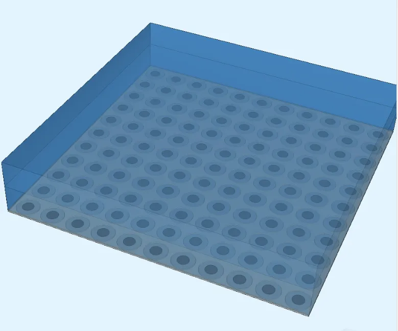
In this example, an 11x11 array of PMUTs (piezoelectric micromachined ultrasonic transducers) is modeled and simulated in the time domain. The array is driven with a voltage pulse and the resulting acoustic beam pattern is computed via Kirchhoff-Helmholtz integral extrapolation on a hemispherical surface in the far field.

PMUT arrays are used in medical ultrasound imaging, range-finding, and gesture recognition. The thin-film stack — SiO₂ substrate, aluminum nitride piezo layer, molybdenum electrodes, and a polysilicon membrane — is the same as in the unit cell tutorial, scaled to a full array with a water load above.

Simulation setup guide

This guide covers the full setup of the 11x11 PMUT array model. The geometry, material, and physics concepts are largely identical to the unit cell tutorial — refer to it for detailed explanations of CSV import, mass rule create, and computed regions.

Step 1 - Variables

Create a new project and start without geometry. Open the Common sidebar, Definitions tab, and import the following variables via Import CSV:

Name,Expression,Description
freq,12e6,Centre excitation frequency (Hz)
V_amp,1.0,Drive voltage amplitude (V)
delay,1.2,Wavelet delay in periods (peak at delay/freq)
pitch,60e-6,Inter-cell pitch (m)
array_n,11,Number of cells per side in the array
cell_d,50e-6,Cavity / cell diameter (m)
bot_elec_d,25e-6,Bottom electrode diameter (m)
t_sio2,2e-6,SiO2 substrate thickness (m)
t_aln,1e-6,AlN piezo layer thickness (m)
t_mo,200e-9,Molybdenum electrode thickness (m)
t_poly,2e-6,Polysilicon elastic layer thickness (m)
c_water,1500,Speed of sound in water (m/s)
lambda_water,c_water / freq,Acoustic wavelength in water (m)
elem_per_wl,6,Mesh elements per wavelength in water
lateral_mesh_size,10e-6,Lateral mesh element size (m)
ppc,25,Time-steps per cycle
dt,1/(freq*ppc),Time-step size (s)
n_cycles,10,Number of excitation cycles to simulate
t_end,n_cycles/freq,Total simulation time (s)
cell_r,cell_d/2,Cell radius (m)
bot_elec_r,bot_elec_d/2,Bottom electrode radius (m)
half_pitch,pitch/2,Half of inter-cell pitch (m)
half_array,array_n * pitch / 2,Half of total array extent (m)
cell_c0,-(array_n-1)/2 * pitch,x/y offset of first cell in grid (m)
eps,0.05e-6,Tolerance for bounding-box region selection (m)
extr_radius,50e-3,Beam pattern extrapolation radius (m)
extr_angle_step,0.5,Beam pattern angular step (degrees)
z_sio2_bot,0,z of SiO2 bottom face (base of stack)
z_sio2_top,t_sio2,z of SiO2 top face / AlN bottom face
z_aln_bot,z_sio2_top,z of AlN bottom face
z_aln_top,z_aln_bot + t_aln,z of AlN top face
z_mo_top_top,z_aln_top + t_mo,z of top Mo electrode upper face
z_poly_top,z_mo_top_top + t_poly,z of polysilicon top face (front face)
z_extr,z_poly_top + lambda_water/2,z of Kirchhoff-Helmholtz extrapolation plane (lambda/2 above front face)
z_water_top,z_poly_top + lambda_water,z of water domain top face

Step 2 - Geometry

Go to the Geometry section. The model consists of 6 boxes (layer stack), 2 cylinders (cavity and bottom electrode for a single cell), a grid operation to replicate them across the array, and a difference operation to carve the cavities.

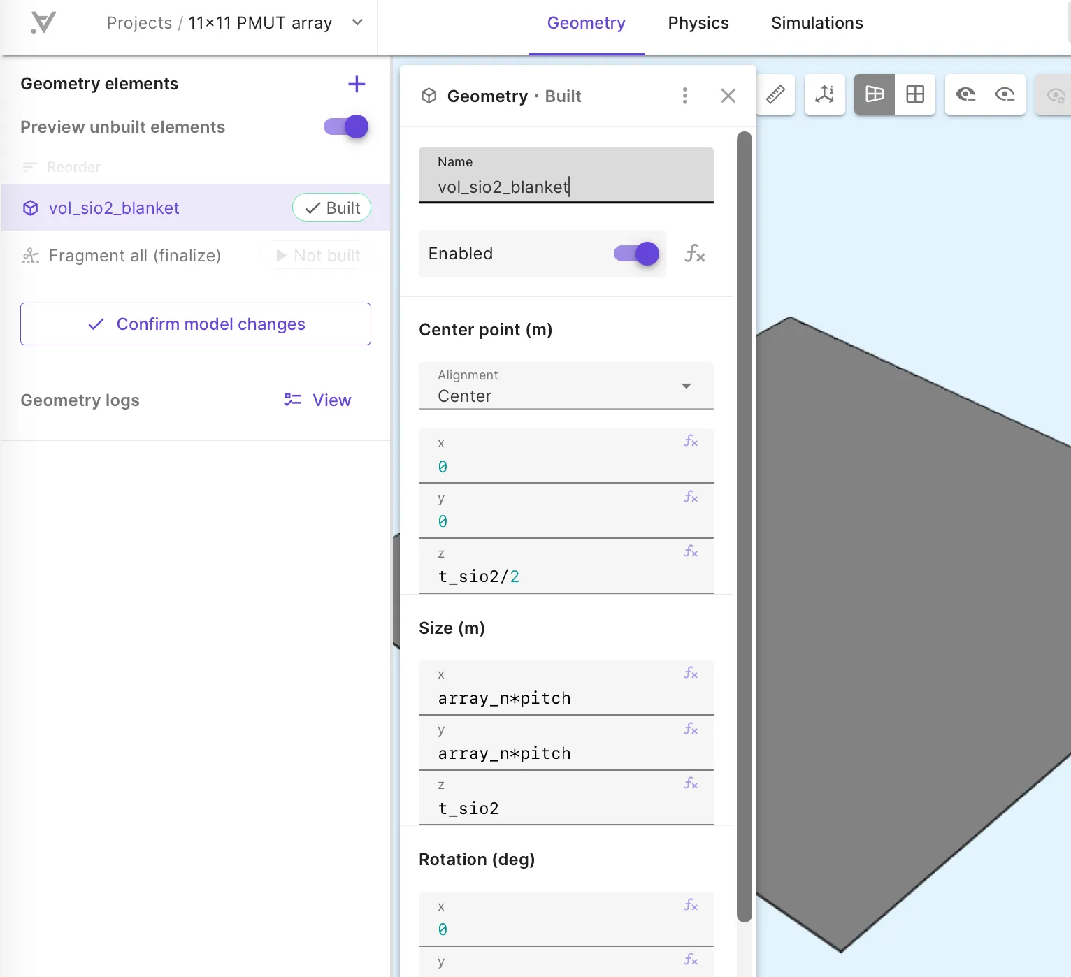
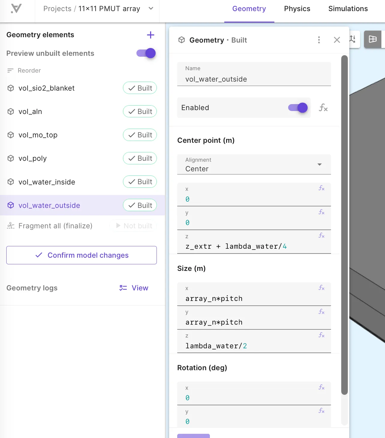
2.1 — Layer boxes

Add 6 Box elements. All share the same X and Y size (array_n*pitch) and differ only in name, center Z, and size Z:

Name	Center Z	Size Z
vol_sio2_blanket	t_sio2/2	t_sio2
vol_aln	z_aln_bot + t_aln/2	t_aln
vol_mo_top	z_aln_top + t_mo/2	t_mo
vol_poly	z_mo_top_top + t_poly/2	t_poly
vol_water_inside	z_poly_top + lambda_water/4	lambda_water/2
vol_water_outside	z_extr + lambda_water/4	lambda_water/2

For all boxes: Center X = 0, Center Y = 0, Size X = array_n*pitch, Size Y = array_n*pitch.

Efficient box creation

Build the first box (vol_sio2_blanket), then copy it and change only the Name, Center Z, and Size Z values for each subsequent layer.

First box

Last box

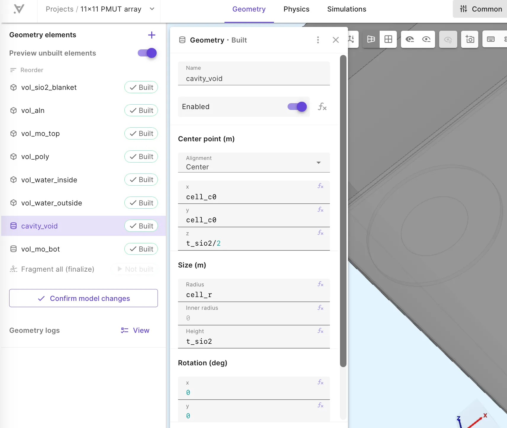
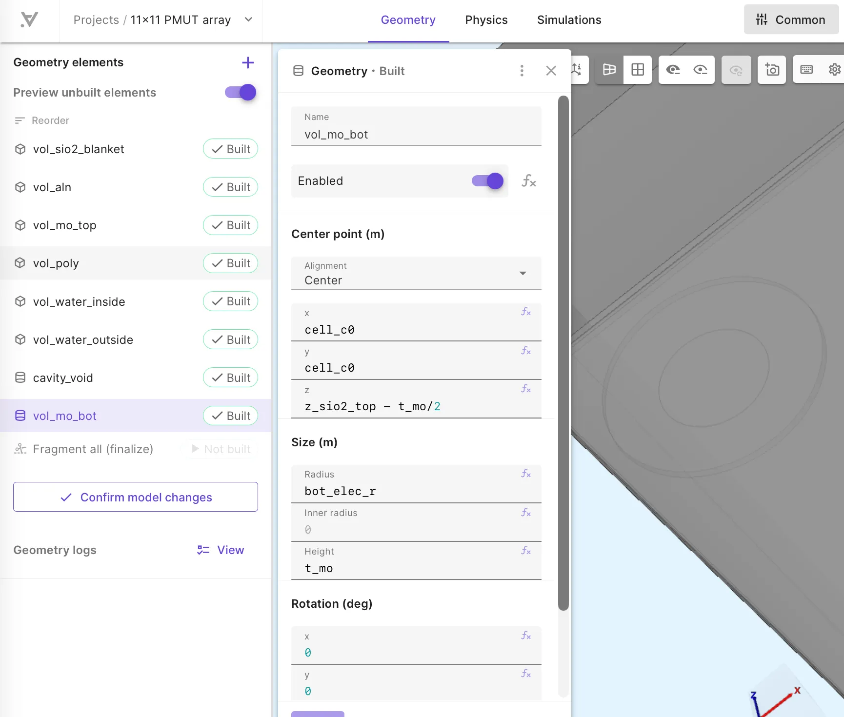
2.2 — Cylinders

Add 2 Cylinder elements for a single unit cell:

Name	Center (X, Y, Z)	Radius	Height
cavity_void	cell_c0, cell_c0, t_sio2/2	cell_r	t_sio2
vol_mo_bot	cell_c0, cell_c0, z_sio2_top - t_mo/2	bot_elec_r	t_mo

First cylinder

Second cylinder

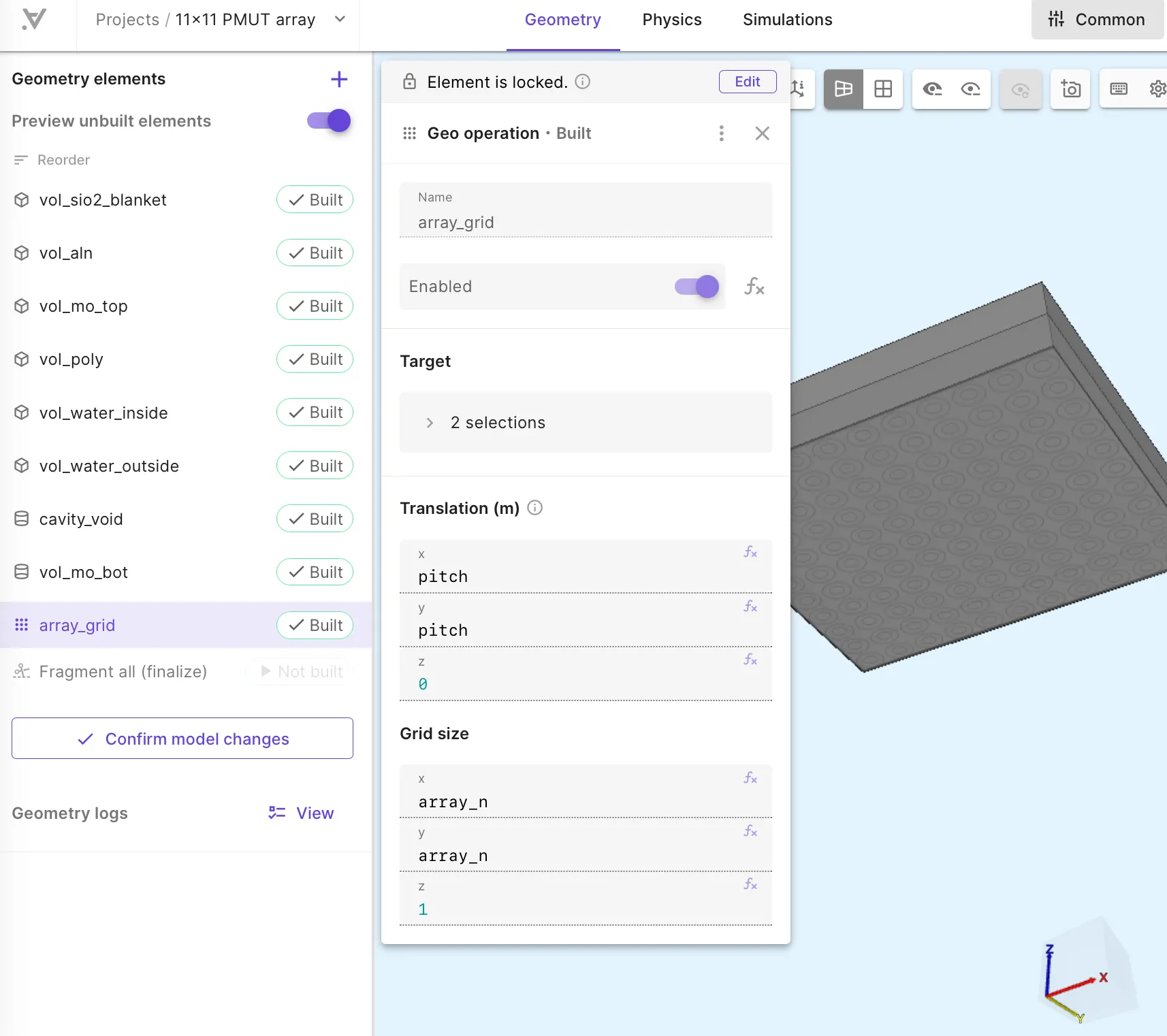
2.3 — Grid operation

Add a Grid operation named array_grid:

Setting	Value
Target	cavity_void, vol_mo_bot
Translation (X, Y, Z)	pitch, pitch, 0
Grid size (X, Y, Z)	array_n, array_n, 1

This replicates both cylinders into an 11x11 pattern across the substrate.

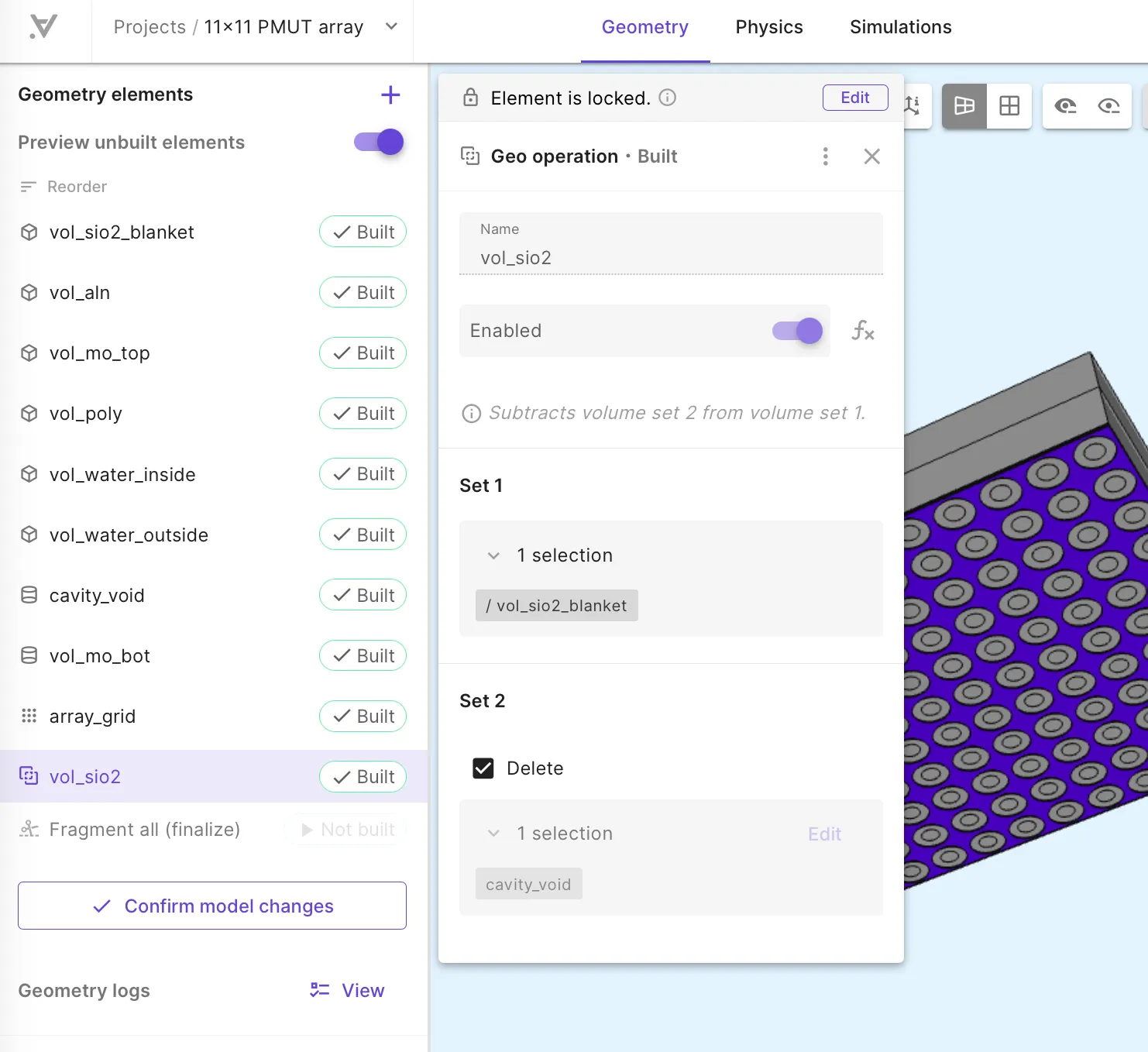
2.4 — Difference operation

Add a Difference operation named vol_sio2:

Setting	Value
Set 1	/vol_sio2_blanket
Set 2	cavity_void
Delete	Checked

This subtracts all 121 cavity cylinders from the SiO₂ blanket and removes the cutter volumes.

Select Confirm model changes (Fragment all).

Step 3 - Material regions

In the Common sidebar, Definitions tab:

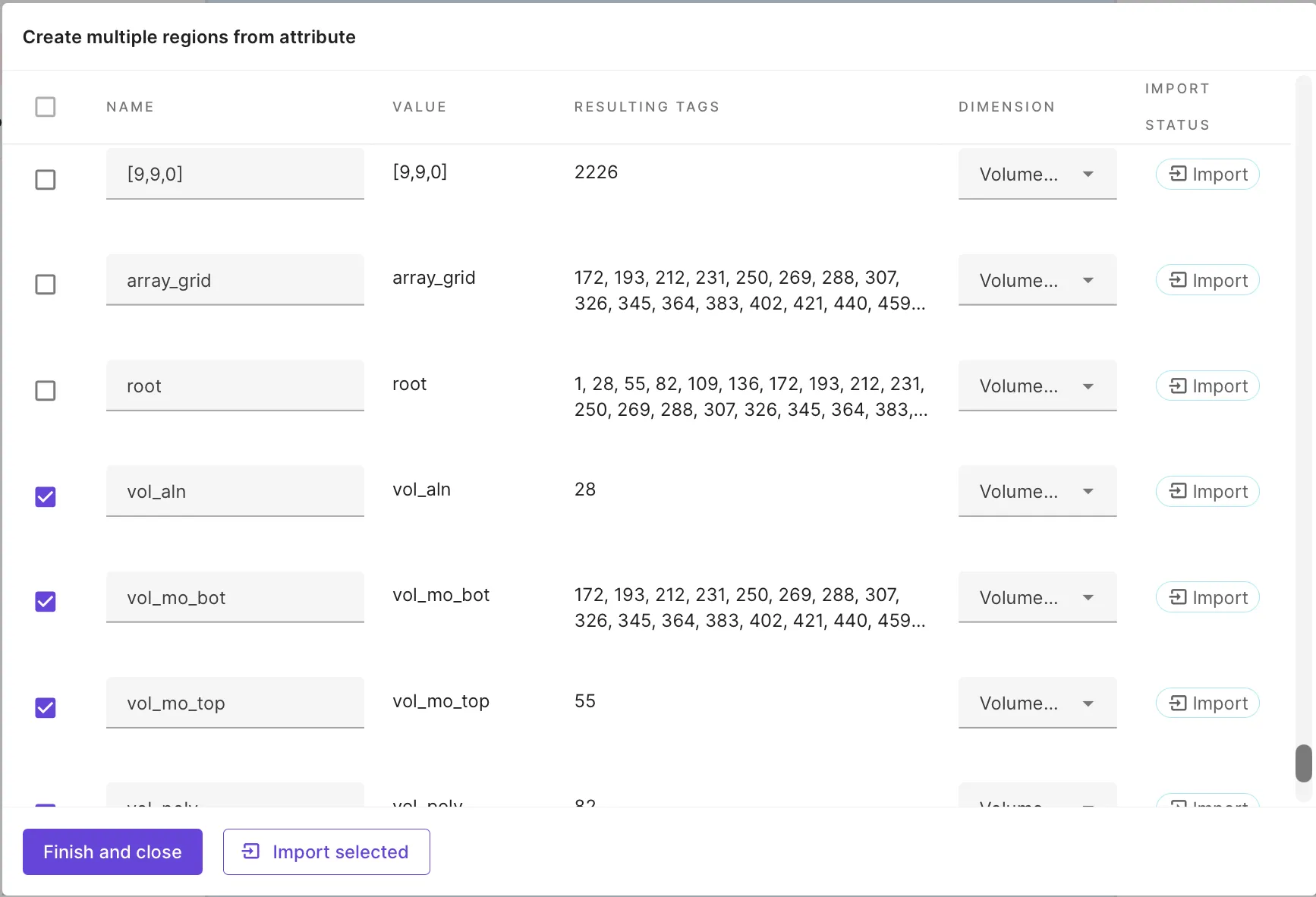
1. Under Regions, use Mass rule create:

   • Attribute: name
   • Entity type: Volume
   • Select only the vol_xxx entries from the bottom of the list (the named geometry volumes).

   

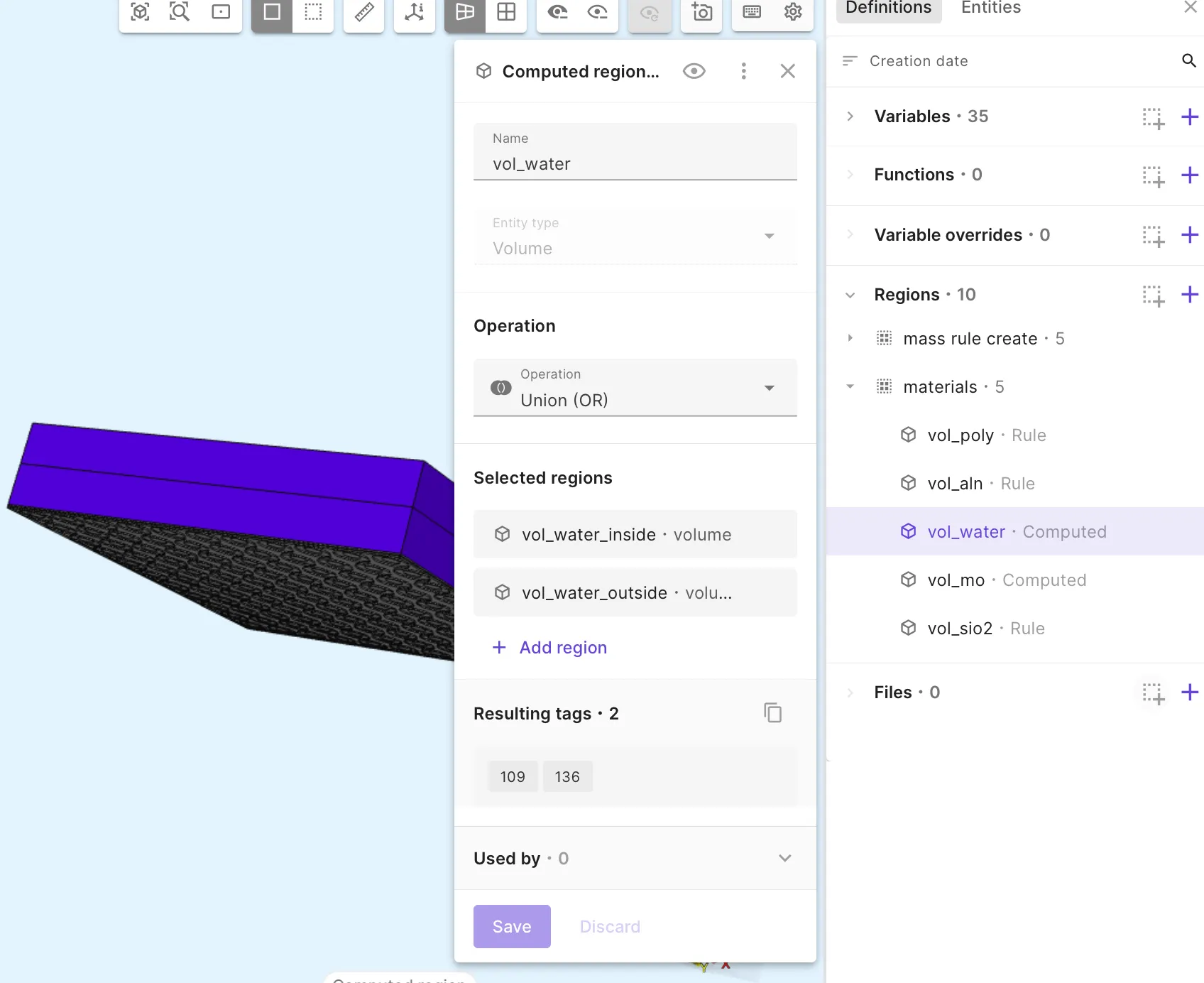
2. Add a Computed region named vol_water (Volume, Union):

   • Regions: vol_water_inside, vol_water_outside

3. Add a Computed region named vol_mo (Volume, Union):

   • Regions: vol_mo_top, vol_mo_bot

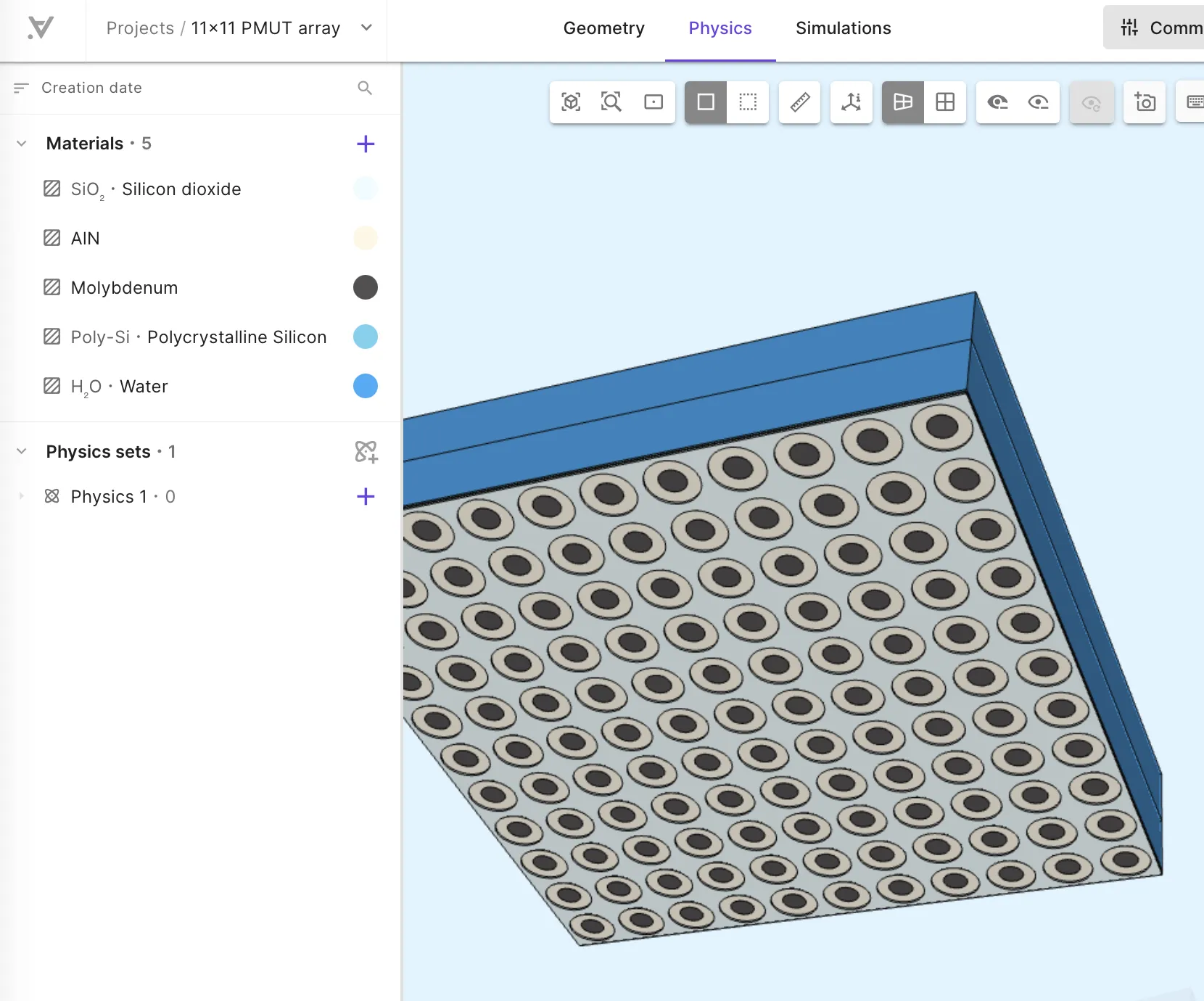
Step 4 - Materials

Go to the Physics section and assign materials from the library:

Material	Target region
Silicon Dioxide	vol_sio2
Aluminum Nitride	vol_aln
Molybdenum	vol_mo
Polycrystalline Silicon	vol_poly
Water	vol_water

Step 5 - Physics regions

Back in the Common sidebar, create the regions needed for boundary conditions and physics targets.

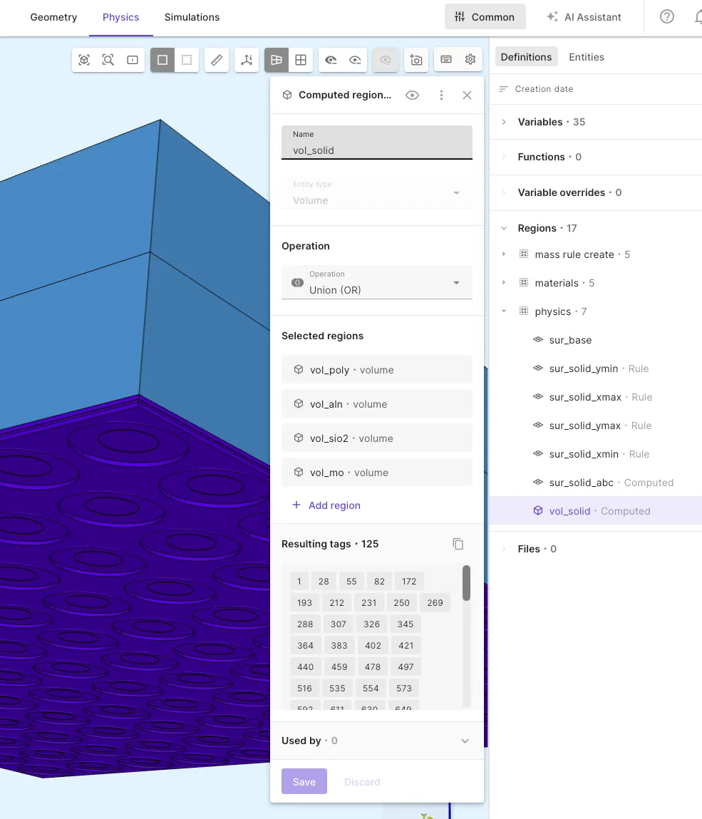
Volume regions

Add a Computed region named vol_solid (Volume, Union):

Regions to union
vol_sio2, vol_aln, vol_poly, vol_mo

Surface regions

Region	Method	Selection hint
sur_base	Surface, manual pick	Bottom face of the stack (SiO₂ base with cavity cutouts)
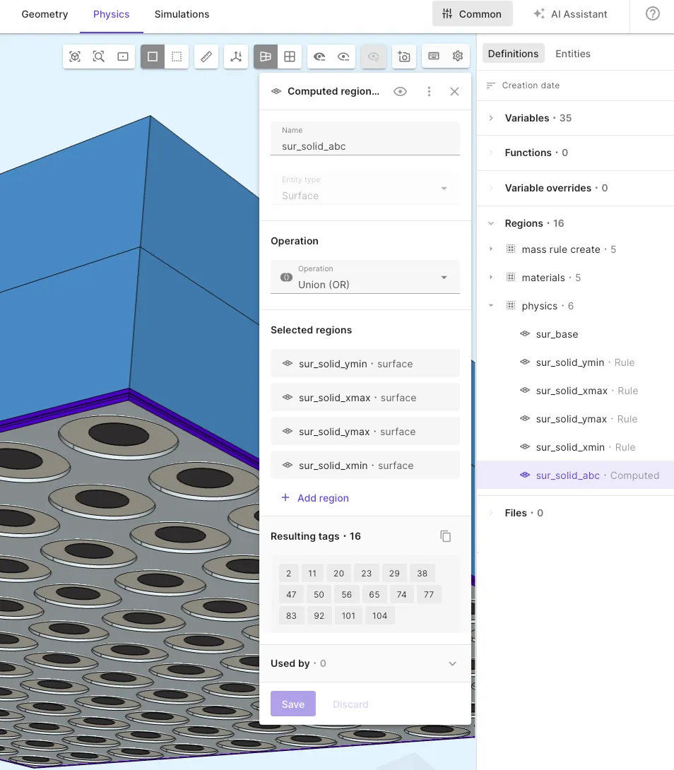
sur_solid_xmin	Rule selector, bounding box + pick similar	Solid surfaces on the x-min face
sur_solid_xmax	Rule selector, bounding box + pick similar	Solid surfaces on the x-max face
sur_solid_ymin	Rule selector, bounding box + pick similar	Solid surfaces on the y-min face
sur_solid_ymax	Rule selector, bounding box + pick similar	Solid surfaces on the y-max face

Then create a Computed region named sur_solid_abc (Surface, Union) combining sur_solid_xmin, sur_solid_xmax, sur_solid_ymin, sur_solid_ymax.

Region	Method	Selection hint
sur_water_abc	Surface, manual pick	Top and lateral outer surfaces of the water domain
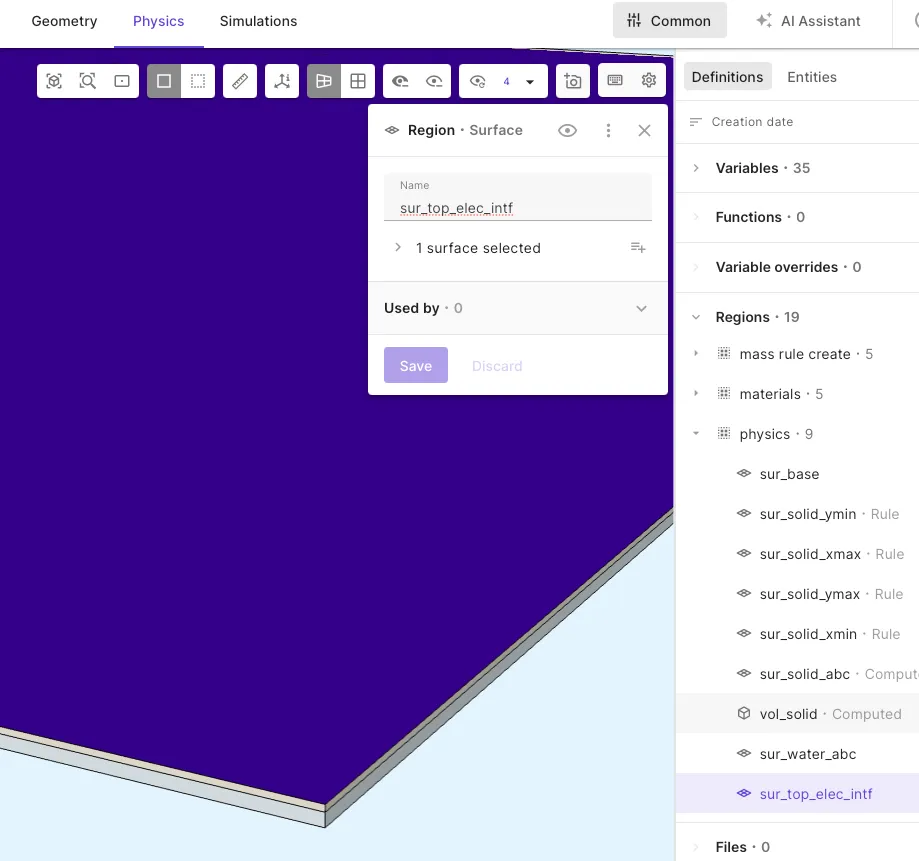
sur_top_elec_intf	Surface, manual pick	Top surface of the AlN layer (hide layers above to access)
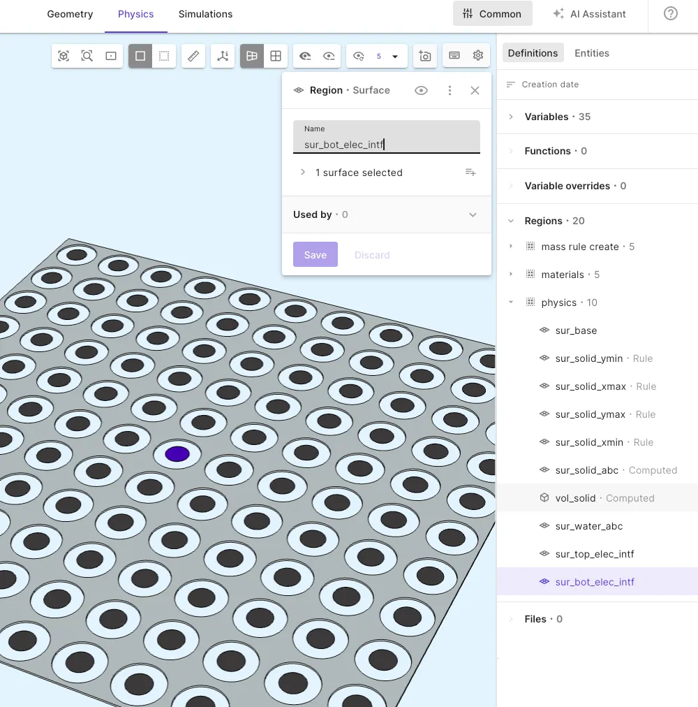
sur_bot_elec_intf	Surface, manual pick	Top surface of the center-most bottom Mo electrode disc

Accessing buried surfaces

Hide layers above the target surface to make it selectable. For sur_top_elec_intf, hide everything above AlN. For sur_bot_elec_intf, continue hiding until the array of cylindrical bottom electrodes is visible, then select the middle-most disc’s top surface.

Top surface of the AlN layer

Top surface of the middle-most electrode disc

Step 6 - Physics

In the Physics section, add three modules to your physics set:

Physics	Target region
Elastic waves	vol_solid
Acoustic waves	vol_water
Electrostatics	vol_aln

Elastic waves interactions

Interaction	Target
Clamp	sur_base
Absorbing boundary	sur_solid_abc
Piezoelectricity	vol_aln

Acoustic waves interactions

Interaction	Target
Acoustic structure	(automatic coupling)
Absorbing boundary	sur_water_abc

Electrostatics interactions

Interaction	Target	Settings
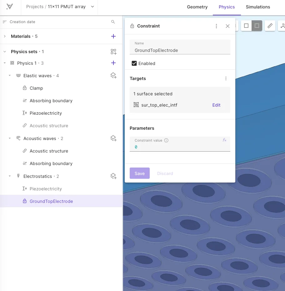
Constraint	sur_top_elec_intf	Value: 0
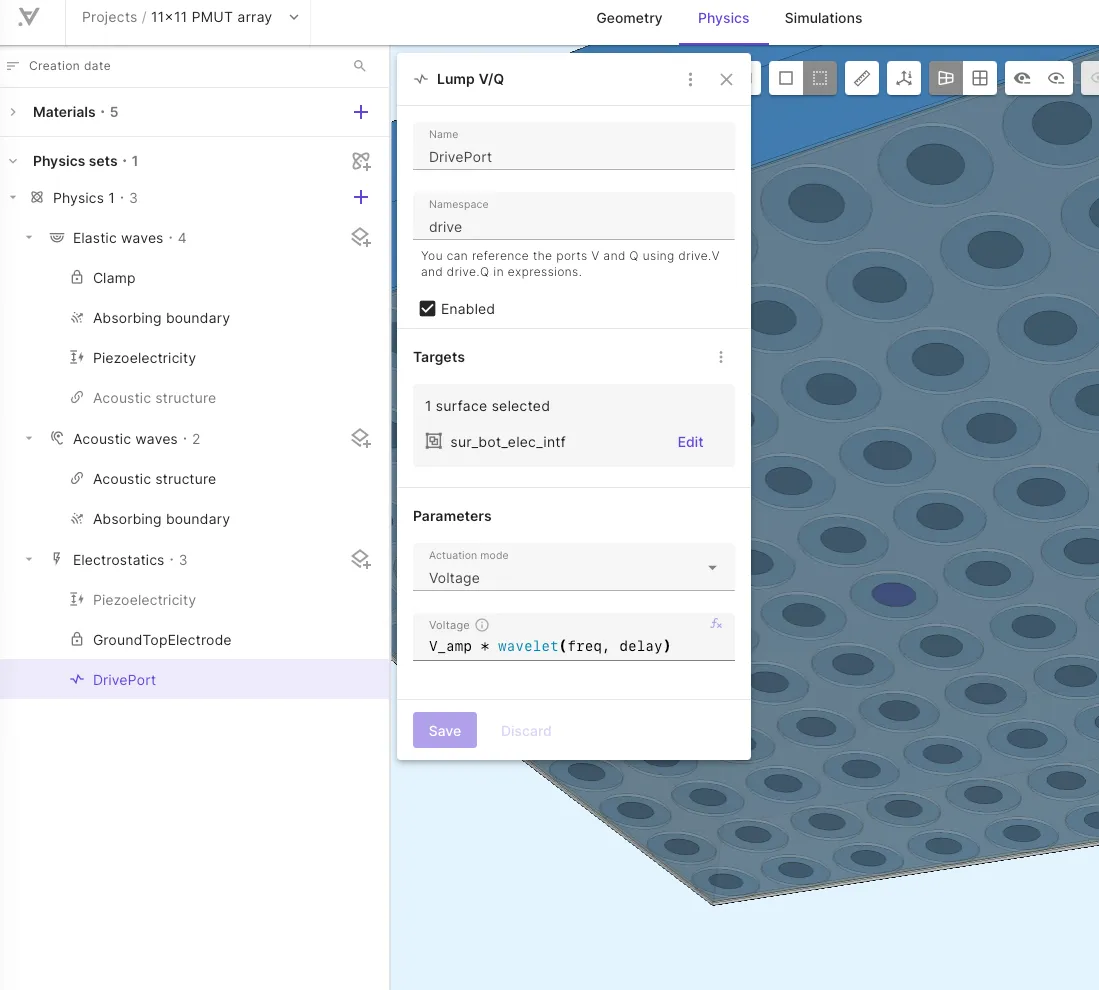
Lump V/Q	sur_bot_elec_intf	Namespace: drive, Mode: Voltage, Value: V_amp * wavelet(freq, delay)

Constraint interaction GroundTopElectrode

Lump V/Q interaction DrivePort

Step 7 - Mesh

In the Simulations section, create a new mesh:

Setting	Value
Autorefine	Disabled
Mesh element size	Absolute
Max size	lateral_mesh_size

Add a Mesh extrusion customization → Simple extrusion:

• Target: select all volumes (results in 7 extrusion layers).
• Sublayer counts (from top to bottom):

Layer	Volume	Sublayers
7	Water outside	3
6	Water inside	3
5	Poly-Si	1
4	Mo top	1
3	AlN	1
2	Mo bottom	1
1	SiO2	1

The two water volumes each get 3 sublayers, giving 6 elements total along the Z-thickness of the combined water domain.

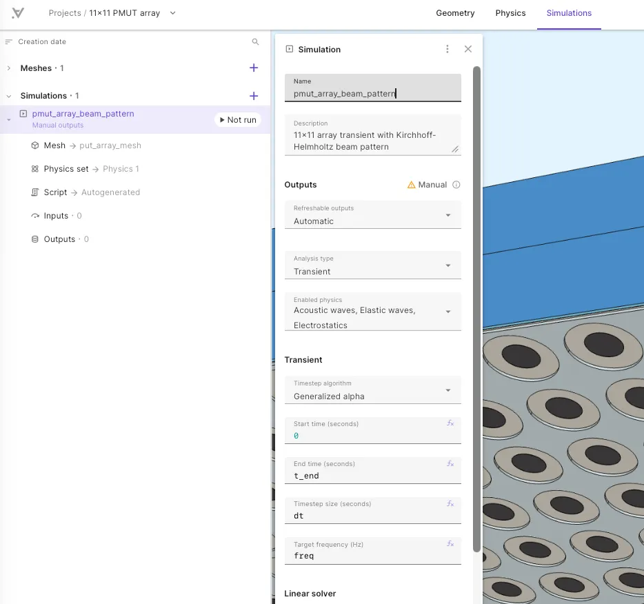
Step 8 - Simulation

Create a new simulation with the following options:

Setting	Value
Name	pmut_array_beam_pattern
Analysis type	Transient
Timestep algorithm	Generalized alpha
Start time	0
End time	t_end
Timestep size	dt
Target frequency	freq

Then, select the mesh you created and add a custom value output called V_drive with expression drive.V.

Script customization

Open the simulation script editor. The script requires two custom sections:

1. Extrapolation helper fields — insert a custom section after the fields are created (after the pressure field fld.p):

# Extrapolation helper fields on the inside water volume
dtp = qs.field("h1")
dtp.setorder(reg.vol_water_inside, 2)
ntp = qs.field("h1")
ntp.setorder(reg.vol_water_inside, 2)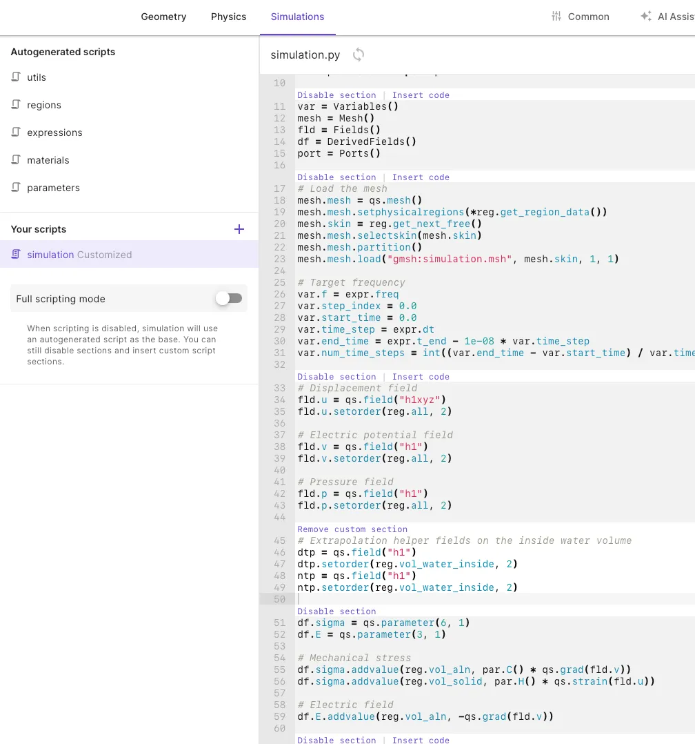

2. Custom time loop — disable the autogenerated SOLVE section and add a custom section with the time loop and Kirchhoff-Helmholtz beam pattern extraction. This requires two additional surface regions in the model:

• sur_extr_plane — the interface between vol_water_inside and vol_water_outside (at z = z_extr)
• sur_front_face — the front face of the solid (poly top, at z = z_poly_top)

Add these as surface regions in the Common sidebar before editing the script.

# --- Custom time loop (replaces disabled SOLVE section) ---
import math

var.step_index = 0.0
var.start_time = 0.0
var.time_step = 1.0 / expr.freq / expr.ppc
var.end_time = expr.n_cycles / expr.freq - 1e-08 * var.time_step

timestepper = qs.genalpha(form, qs.vec(form), qs.vec(form))
timestepper.settolerance(1e-05)
timestepper.setrelaxationfactor(-1)
qs.settime(var.start_time)

extr_times = [var.start_time]
extr_pdtpntp = [[fld.p.copy(), dtp.copy(), ntp]]

while qs.gettime() < var.end_time:
    timestepper.allnext(relrestol=1e-06, maxnumit=1000, timestep=var.time_step, maxnumnlit=1000)

    dtp.setvalue(reg.sur_extr_plane, qs.dt(fld.p))
    ntp = form.allneumann(reg.sur_extr_plane, reg.vol_water_inside, fld.p)
    extr_times.append(qs.gettime())
    extr_pdtpntp.append([fld.p.copy(), dtp.copy(), ntp])

    var.discrete = qs.evaluate(port.drive.V)
    qs.setoutputvalue("V_drive", var.discrete, qs.gettime())
    var.discrete = qs.evaluate(port.drive.Q)
    qs.setoutputvalue("Q_drive", var.discrete, qs.gettime())
    var.discrete = qs.evaluate(qs.dt(port.drive.Q))
    qs.setoutputvalue("I_drive", var.discrete, qs.gettime())
    var.discrete = qs.allaverage(reg.sur_front_face, fld.p, 3)
    qs.setoutputvalue("p_avg_front", var.discrete, qs.gettime())

    var.step_index += 1

# --- Post-loop: Kirchhoff-Helmholtz beam pattern ---
c_w = mat.water.c()
rho_w = mat.water.rho()
radius = expr.extr_radius
angle_step_deg = expr.extr_angle_step
z_front = expr.z_poly_top

angles_deg = []
a = -90.0
while a <= 90.0 + 1e-9:
    angles_deg.append(a)
    a += angle_step_deg
n_angles = len(angles_deg)

extr_delay = radius / c_w
output_times = [t + extr_delay - 1.0 / expr.freq for t in extr_times]

qs.printonrank(0, f"Beam pattern: {n_angles} angles, radius={radius*1e3:.1f} mm")

max_pres = []
pres_on_axis = None

for i, ang_deg in enumerate(angles_deg):
    ang_rad = ang_deg * math.pi / 180.0
    coord = [radius * math.sin(ang_rad), 0.0, z_front + radius * math.cos(ang_rad)]
    if i % 30 == 0:
        qs.printonrank(0, f"  angle {i}/{n_angles}: {ang_deg:.1f} deg")
    pres = qs.helmholtzkirchhoff(
        form, reg.sur_extr_plane, reg.vol_water_inside, fld.p,
        c_w, rho_w, coord, output_times, extr_times, extr_pdtpntp,
    )
    max_pres.append(max(abs(p) for p in pres))
    if abs(ang_deg) < 1e-9:
        pres_on_axis = pres

qs.setoutputvalue("extr_times_0deg", output_times)
qs.setoutputvalue("extr_pres_0deg", pres_on_axis)
qs.setoutputvalue("angles_deg", angles_deg)
qs.setoutputvalue("max_pres", max_pres)

p_max_global = max(max_pres) if max(max_pres) > 0 else 1e-30
db_pattern = [20.0 * math.log10(p / p_max_global) if p > 0 else -100.0 for p in max_pres]
qs.setoutputvalue("beam_pattern_dB", db_pattern)

qs.printonrank(0, f"Peak pressure: {p_max_global:.4e} Pa at on-axis")

The simulation outputs drive voltage, charge, current, and front-face average pressure at each time step. After the time loop completes, the Kirchhoff-Helmholtz integral computes the beam pattern in dB across all angles from -90° to +90°.

Results

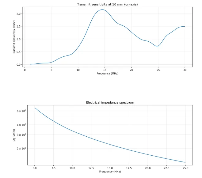
Transmit sensitivity and impedance

The transmit sensitivity spectrum (evaluated at the 50 mm extrapolation radius) peaks around 13–15 MHz, consistent with the fundamental flexural resonance of the membrane stack. Compared to the single unit cell, the array produces a higher on-axis sensitivity due to constructive interference from the 121 elements. The electrical impedance remains predominantly capacitive and monotonically decreasing with frequency — expected for a thin AlN film well below its thickness-mode resonance.

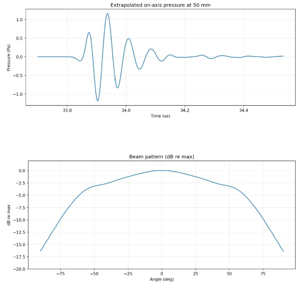
Beam pattern and far-field pressure

The extrapolated on-axis pressure waveform at 50 mm shows a clean Ricker-like pulse arriving at roughly 33.9 µs (the acoustic travel time from the array face to the observation point). The pulse amplitude reaches about 1.2 Pa, confirming effective focusing by the planar array.

The beam pattern shows a well-defined main lobe centered at 0° with a −3 dB half-angle of approximately ±40°. Side lobes appear near ±50–60°, suppressed by about 3 dB relative to the main lobe. At grazing angles beyond ±75°, the response drops by 15 dB or more. This broad beam is characteristic of an unfocused planar array at a frequency where the array aperture is only a few wavelengths across.