
Piezocomposite transducer
Prerequisites: complete the PMUT Unit cell - Ultrasound 001 tutorial first.
In this example, a piezocomposite ultrasound transducer is simulated. Their main application is in medicine, where they are used for ultrasound imaging and medical therapeutics. Other applications include sonar and non-destructive testing.
The model captures a single element of a 1-3 piezocomposite linear array. The piezocomposite element combines a soft PZT with an epoxy filler with a 40% volume fraction. It is driven with a short voltage pulse to allow the wideband behaviour, or impulse response, of the device to be captured. Key outputs are:
- Drive voltage and current
- Pressure in the load
- Electrical impedance
Demo project: Piezocomposite demo V1
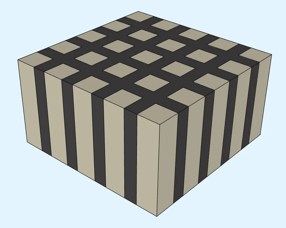
Simulation setup guide
Section titled “Simulation setup guide”Here you’ll find a simplified, example case level guide for setting up a piezocomposite transducer simulation in Quanscient Allsolve.
Step 1 - Define variables
Section titled “Step 1 - Define variables”Start out in the Common sidebar by defining variables.
| Name | Description | Expression |
|---|---|---|
| frequency | Frequency [Hz] | 1.25e6 |
| ncycles | Number of cycles | 5 |
| npillars | Number of pillars | 5 |
| thick_comp | Composite thickness [m] | 1e-3 |
| kerf | Cut width [m] | 0.15e-3 |
| pitch | Distance between cuts [m] | 0.4e-3 |
| pillar | Pillar width [m] | pitch-kerf |
| width | Element width [m] | npillars*pitch - kerf |
| minvel | Minimum acoustic wave velocity in the model (epoxy shear) [m/s] | 1110 |
| epw | Number of elements per wavelength | 4 |
| element_size | Mesh element max size [m] | minvel/freq/epw |
You can import the variables as a CSV file:
Name,Expression,Descriptionfreq,1.25e6,Frequency [Hz]ncycles,5,Number of cyclesnpillars,5,Number of pillarsthick_comp,1e-3,Composite thickness [m]kerf,0.15e-3,cut width [m]pitch,0.4e-3,Distance between cuts [m]pillar,pitch-kerf,pillar width [m]width,npillars*pitch-kerf,Element width [m]minvel,1110,Minimum acoustic wave velocity in the model (epoxy shear) [m/s]epw,4,Number of elements per wavelengthelement_size,minvel/freq/epw,Mesh element max size [m]Step 2 - Build the geometry
Section titled “Step 2 - Build the geometry”-
Start building the model geometry by adding Box elements with Alignment = Corner:
Name Element type Corner point [m] Size [m] Rotation [deg] pzt Box X: 0X: widthX: 0Y: 0Y: widthY: 0Z: 0Z: thick_compZ: 0Name Element type Corner point [m] Size [m] Rotation [deg] cut x Box X: 0X: widthX: 0Y: pillarY: kerfY: 0Z: 0Z: thick_compZ: 0Name Element type Corner point [m] Size [m] Rotation [deg] cut y Box X: pillarX: kerfX: 0Y: 0Y: widthY: 0Z: 0Z: thick_compZ: 0 -
Use the Translate operation to copy the cuts in X and Y directions:
Name Element type Target Translation [m] Copy Repeat count copy x Translation cut y X: pitchYes npillars - 2Y: 0Z: 0Name Element type Target Translation [m] Copy Repeat count copy y Translation cut x X: 0Yes npillars - 2Y: pitchZ: 0 -
Use the Union operation to merge all the multiplied cuts to a single volume:
Name Element type Target combine polymer Union copy x and copy y assemblies (all cut volumes) -
Confirm model changes.
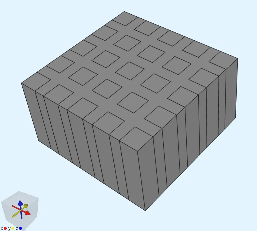
Finished geometry:
Step 3 - Define the materials
Section titled “Step 3 - Define the materials”Go to the Physics section to define model materials.
Material 1 - PZT
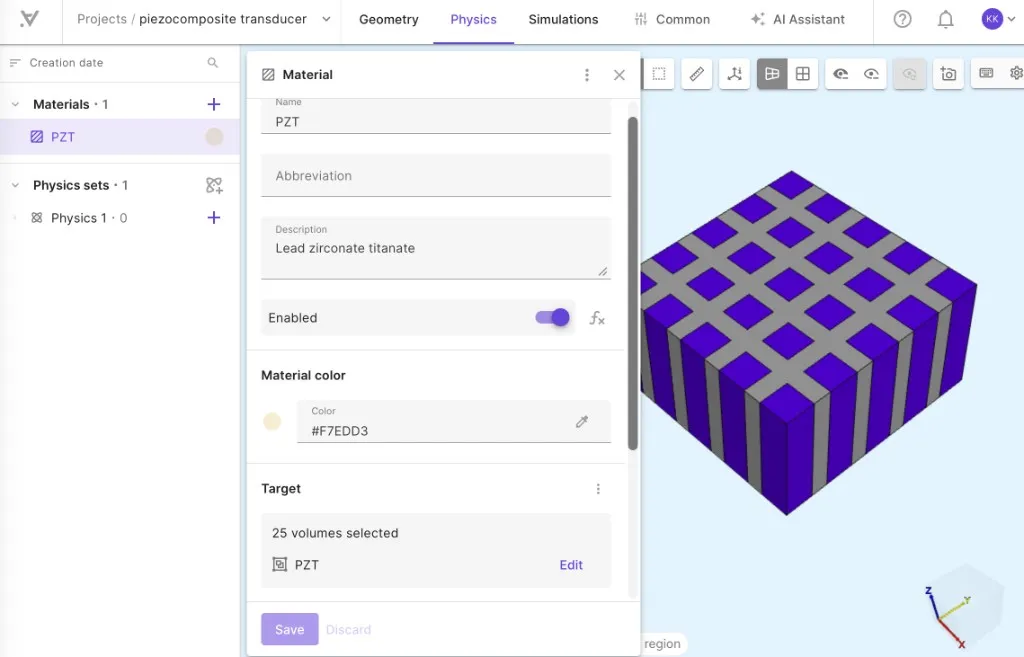
Section titled “Material 1 - PZT”Add PZT from the library and assign it to the piezoelectric pillars:
- Go to Target -> Pick with rule -> Select all volumes as target
- Remove the epoxy filler volume from the selection by clicking on the model view.
- Add the final target with 25 pillars as a region.
Material 2 - Epoxy
Section titled “Material 2 - Epoxy”-
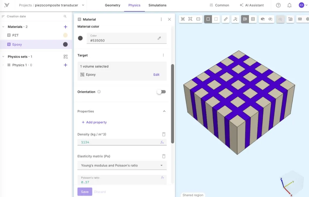
Create a new material for the epoxy filler:
Material Target Epoxy Polymer filler volume -
Define material properties for Epoxy:
Property Value Units Density 1134Elasticity matrix Poisson’s ratio: 0.37Young’s modulus: 3.831e9Electric permittivity 4*epsilon0 -
Add the target as a region.
Step 4 - Define the physics
Section titled “Step 4 - Define the physics”The Elastic waves and Electrostatics physics are required for this example.
Add both of them to your physics set before defining interactions, in order to couple them together.
Physics 1 - Elastic waves
Section titled “Physics 1 - Elastic waves”- Let elastic waves target default to the whole geometry.
- Add the Elastic waves - Electrostatics coupling
Piezoelectricity.- Select the
PZTregion as target.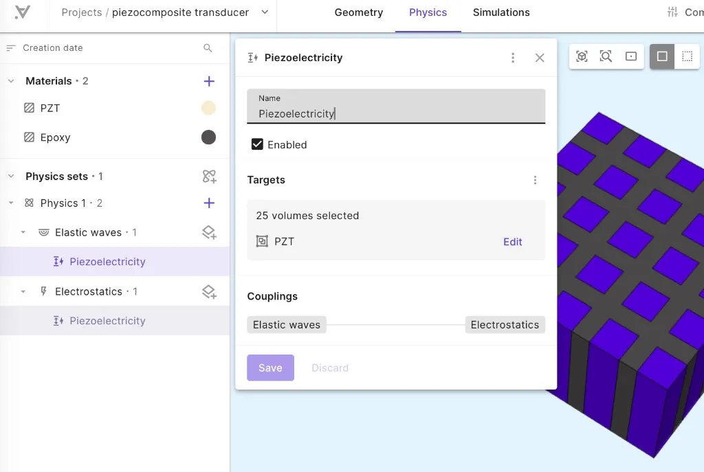
- Select the
Physics 2 - Electrostatics
Section titled “Physics 2 - Electrostatics”-
Let Electrostatics target default to the whole geometry.
-
Add a
Constraintinteraction which acts as a ground on the bottom surface:Interaction Target Constraint value ConstraintBottom surface of the whole element 0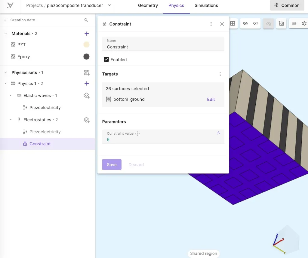
-
Add a
Lump V/Qinteraction which drives a voltage on the top surface withwavelet:Interaction Target Voltage Lump V/QTop surface of the element wavelet(frequency, 1.2)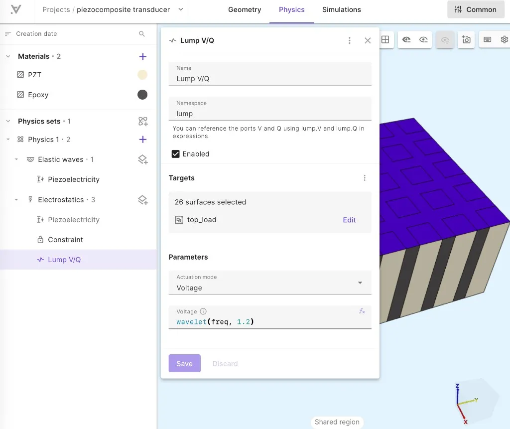
Step 5 - Generate a mesh
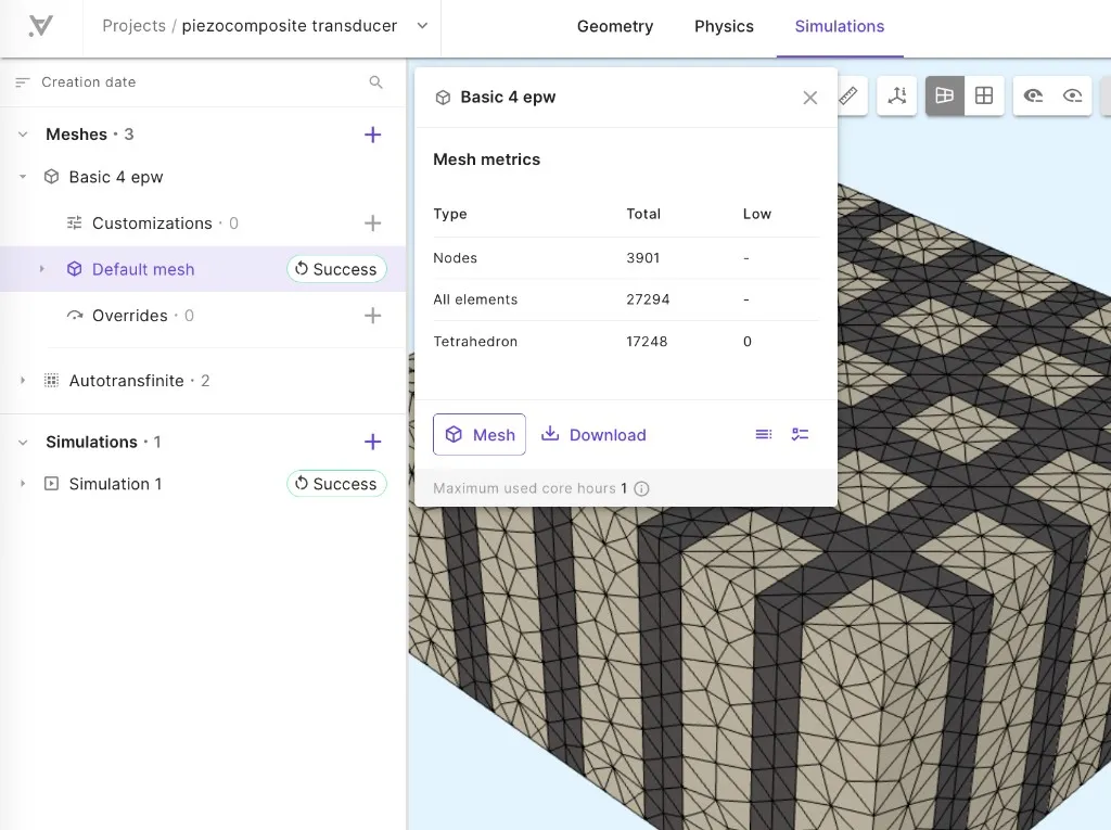
Section titled “Step 5 - Generate a mesh”Go to the Simulations section to create a new mesh with basic settings.
- In mesh settings, convert mesh element size to Absolute.
- Set mesh element max size to
element_size(defined asminvel/freq/epwin Step 1). - Run meshing.
- Check the preview:
Optional: Mesh refinement based on material
Section titled “Optional: Mesh refinement based on material”Using a single mesh element max size for the model is OK, but can be inefficient if you have a large area of ‘fast’ material which will be overmeshed. A Mesh refinement customization can be added for each material independently to maintain accuracy and efficiency.
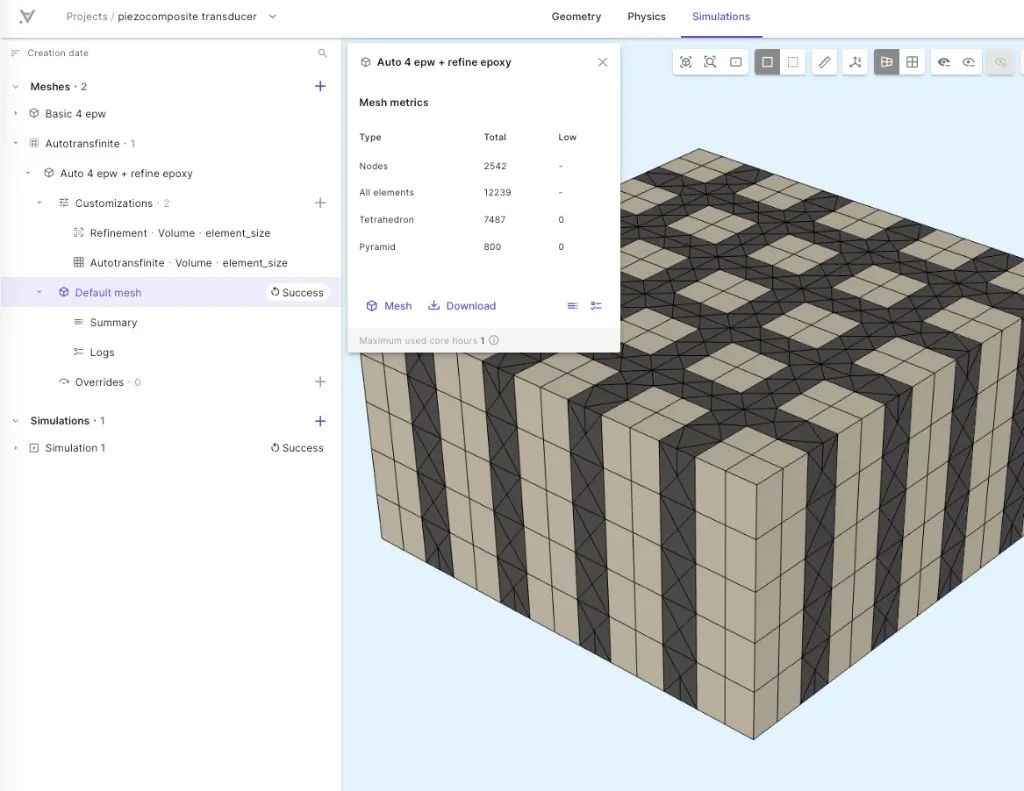
Optional: Autotransfinite meshing
Section titled “Optional: Autotransfinite meshing”You can also create a mesh using an Autotransfinite mesh customization. Autotransfinite is designed for blocky geometries laid out in a XYZ-aligned grid, so it is a great option for the PZT pillars in this case.
Step 6 - Simulate
Section titled “Step 6 - Simulate”In the Simulations section, create a new simulation:
-
Set Analysis type to
Transient. -
Select timestepping options:
Timestep algorithm Start time [s] End time [s] Timestep size [s] Generalized alpha0ncycles/freq1/freq/20 -
Select a mesh.
-
Add Outputs:
Output type Name Output expression Skin only Field Displacement field u uYes Custom value Voltage lump.VCustom value Current dt(lump.Q)
Your simulation is now ready to run.
Step 7 - Results
Section titled “Step 7 - Results”In the Simulations section, you can add plots to see value output results and visualizations to see field output results.
-
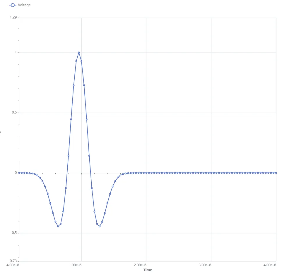
Voltage:
-
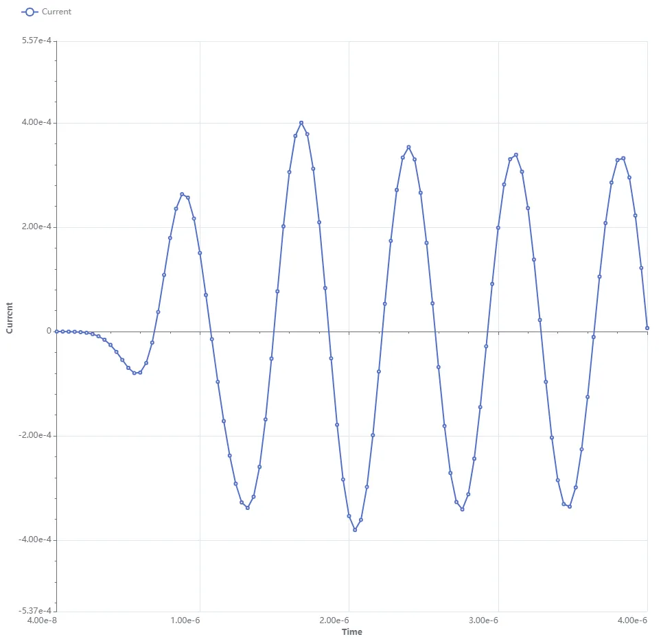
Current:
-
Displacement field: