Coaxial tee S-parameters - RF 004

What you’ll learn

• How to build a coaxial T-junction geometry using cylinders and boolean operations (Union, Difference).
• How to configure three eigenmode ports on a coaxial waveguide and extract S-parameters from a 3-port power splitter.
• How to run a harmonic frequency sweep and visualize the electric field distribution inside the junction.

Prerequisites: complete RF 001 — Eigenmode ports and S-parameters first — it introduces eigenmode ports, S-parameters, and the harmonic sweep workflow used here.

Demo project

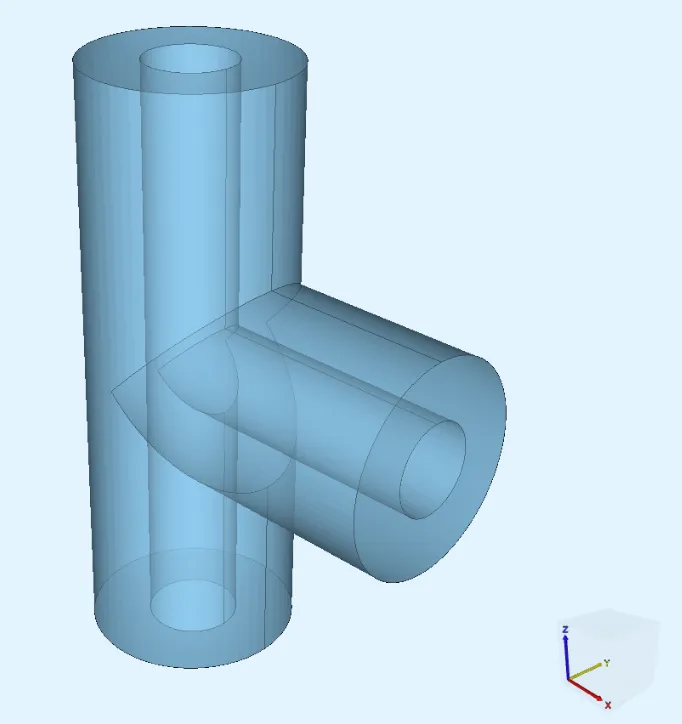
A coaxial tee is a three-port power splitter formed by joining a branch coaxial line at a right angle to the midpoint of a main coaxial line. Power entering any port splits between the other two. The geometry dimensions give a characteristic impedance $Z_0 = 60\,\ln(r_\text{outer}/r_\text{pin}) \approx 50\,\Omega$ on every arm.

This tutorial reproduces the coaxial tee benchmark from ANSYS HFSS Getting Started Workshop 4.1 ¹ and compares S-parameter results across the 1–10 GHz band.

---

Simulation setup guide

Step 1 - Import variables

In the Common sidebar, open the Variables panel, and import the following variables as CSV:

Name,Expression,Description
outer_r,0.00189,Outer conductor inner radius [m]
pin_r,0.000821,Inner conductor (pin) radius [m]
main_len,0.0108,Main arm total length [m]
branch_len,0.0054,Branch arm length [m]
tol,1e-4,Region-selection tolerance [m]
freq,1000000000.0,Operating frequency [Hz]

Name	Description	Expression
outer_r	Outer conductor inner radius [m]	0.00189
pin_r	Inner conductor (pin) radius [m]	0.000821
main_len	Main arm total length [m]	0.0108
branch_len	Branch arm length [m]	0.0054
tol	Region-selection tolerance [m]	1e-4
freq	Operating frequency [Hz]	1000000000.0

Step 2 - Build the geometry

Go to the Geometry section. Build the coaxial tee from four cylinders and three boolean operations.

1. Add a new Cylinder named main_outer:

   Setting	Value
   Radius	outer_r
   Height	main_len

2. Copy main_outer and edit the copy:

   Setting	Value
   Name	main_pin
   Radius	pin_r

3. Add a new Cylinder named branch_outer:

   Setting	Value
   Center X	branch_len / 2
   Radius	outer_r
   Height	branch_len
   Rotation Y	90

4. Copy branch_outer and edit the copy:

   Setting	Value
   Name	branch_pin
   Radius	pin_r

5. Add a Union operation named outer_union:

   Setting	Value
   Set	/ main_outer, / branch_outer

6. Add a Union operation named pin_union:

   Setting	Value
   Set	/ main_pin, / branch_pin

7. Add a Difference operation named air_domain:

   Setting	Value
   Set 1	/ outer_union
   Set 2	/ pin_union
   Delete	Yes

8. Select Confirm model changes.

Step 3 - Create regions

Return to the Common sidebar and open the Regions panel. Create the following regions:

1. Add a volume region named air_volume targeting the entire air domain volume.

2. Add a surface region named port1 targeting the main cylinder bottom surface (Z-min face).

3. Add a surface region named port2 targeting the branch cylinder end surface (X-max face).

4. Add a surface region named port3 targeting the main cylinder top surface (Z-max face).

5. Add a surface region named all_surfaces targeting all surfaces of the air domain.

6. Add a computed surface region named pec_walls:

   Setting	Value
   Operation	Difference
   A	all_surfaces
   B	port1, port2, port3

   This selects all outer walls except the three port faces.

Step 4 - Apply materials

Go to the Physics section. Assign the Air material from the library to the air_volume region.

Step 5 - Define the physics

In the Physics section, add the Electromagnetic waves physics.

1. Add a Perfect conductor interaction:

   Setting	Value
   Name	PEC walls
   Target	pec_walls

2. Add an Eigenmode port interaction:

   Setting	Value
   Name	Port 1
   Target	port1
   Number of eigenmodes to find	5
   Eigenmode index	0
   Target eigenvalue	Effective refractive index
   Effective refractive index	1
   Drive	Yes
   Driving signal	sin(2*pi*freq*t)

3. Copy Port 1 and edit the copy:

   Setting	Value
   Name	Port 2
   Target	port2

4. Copy Port 2 and edit the copy:

   Setting	Value
   Name	Port 3
   Target	port3

Why five eigenmodes?

The coaxial cross-section supports one TEM mode at these frequencies. Requesting five eigenmodes ensures the solver finds the TEM mode reliably, even though only eigenmode index 0 (the fundamental) is used. Unused higher-order modes are discarded automatically.

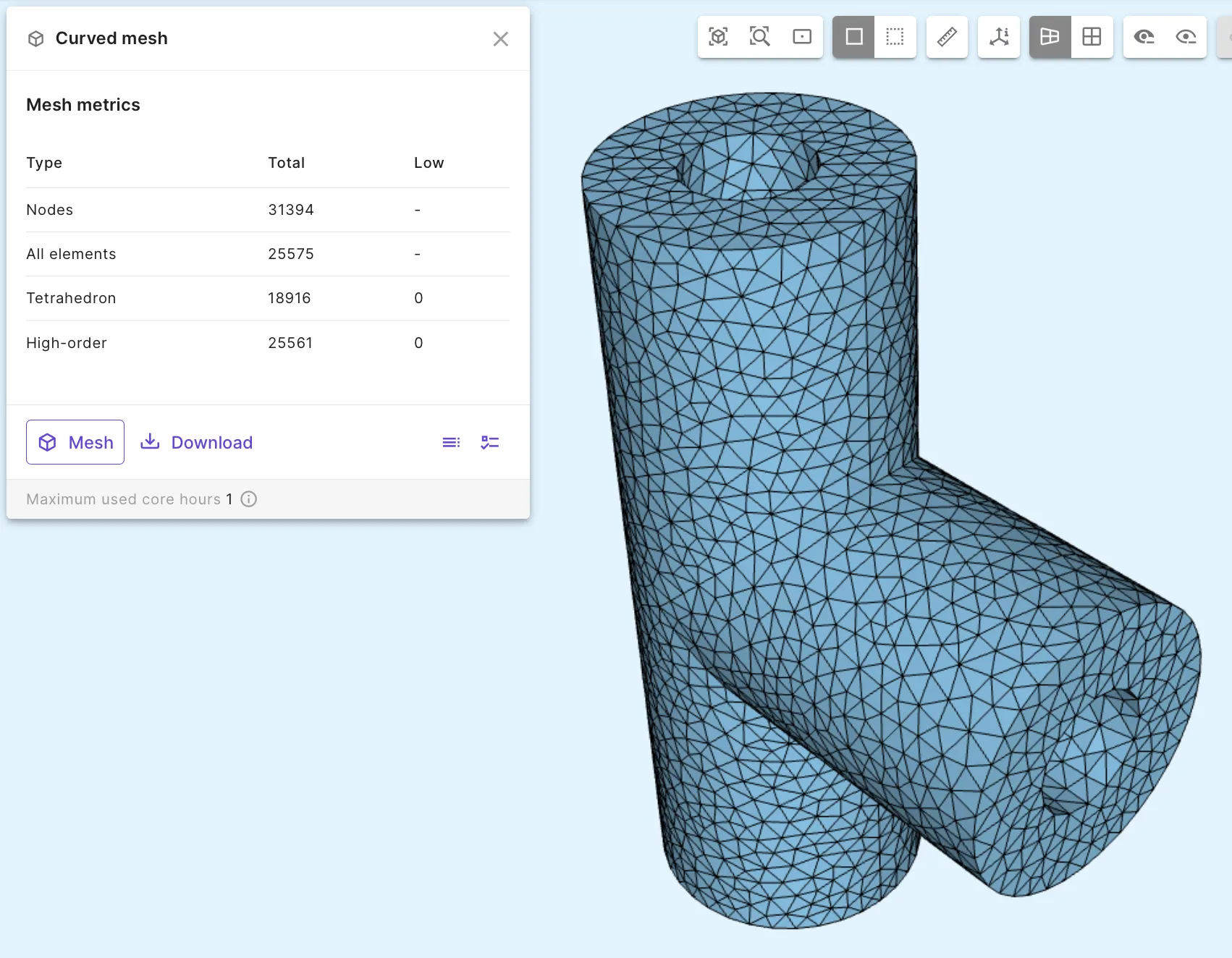
Step 6 - Generate the mesh

Go to the Simulations section and create a new mesh named curved mesh. Configure the following settings:

Setting	Value
Mesh element size	Absolute
Min. size	0.0001
Max. size	0.0005
Curvature enhancement	0.2
Curved mesh	Yes

Step 7 - Set up and run the simulation

In the Simulations section, add a new simulation:

Setting	Value
Name	Coax Tee S-Parameters
Description	Harmonic EM simulation — S-parameters and E-field
Analysis type	Harmonic
Fundamental frequency	freq
Number of FFT samples	3
Solver mode	Iterative solver
Mesh	curved mesh

Inputs:

1. In the Common sidebar, add a variable override for freq.
2. Set the override expression to linspace(1e9, 1e10, 10).
3. Add this override as an input to the simulation.

Outputs:

1. Add S-parameters.
2. Add Electric field (2nd harmonic).
   • Rename to E-field.
   • Turn on Skin only.

Run the simulation.

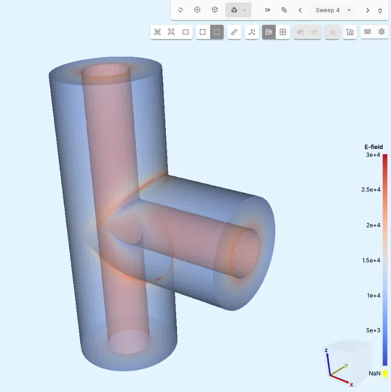
Step 8 - Results

After the simulation completes, add a visualization for the E-field output and browse through sweep steps:

E-field distribution in the coaxial tee for sweep step 4

Plot the S-parameters to see the frequency-dependent power split:

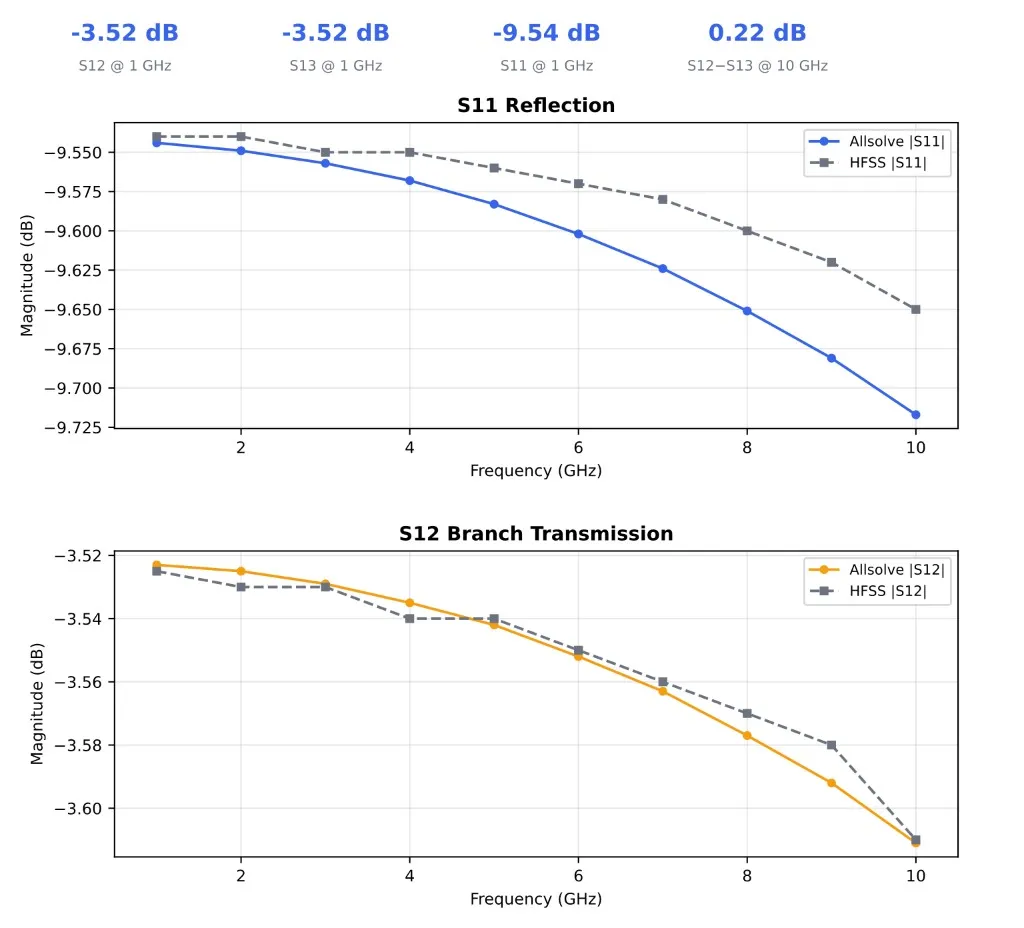
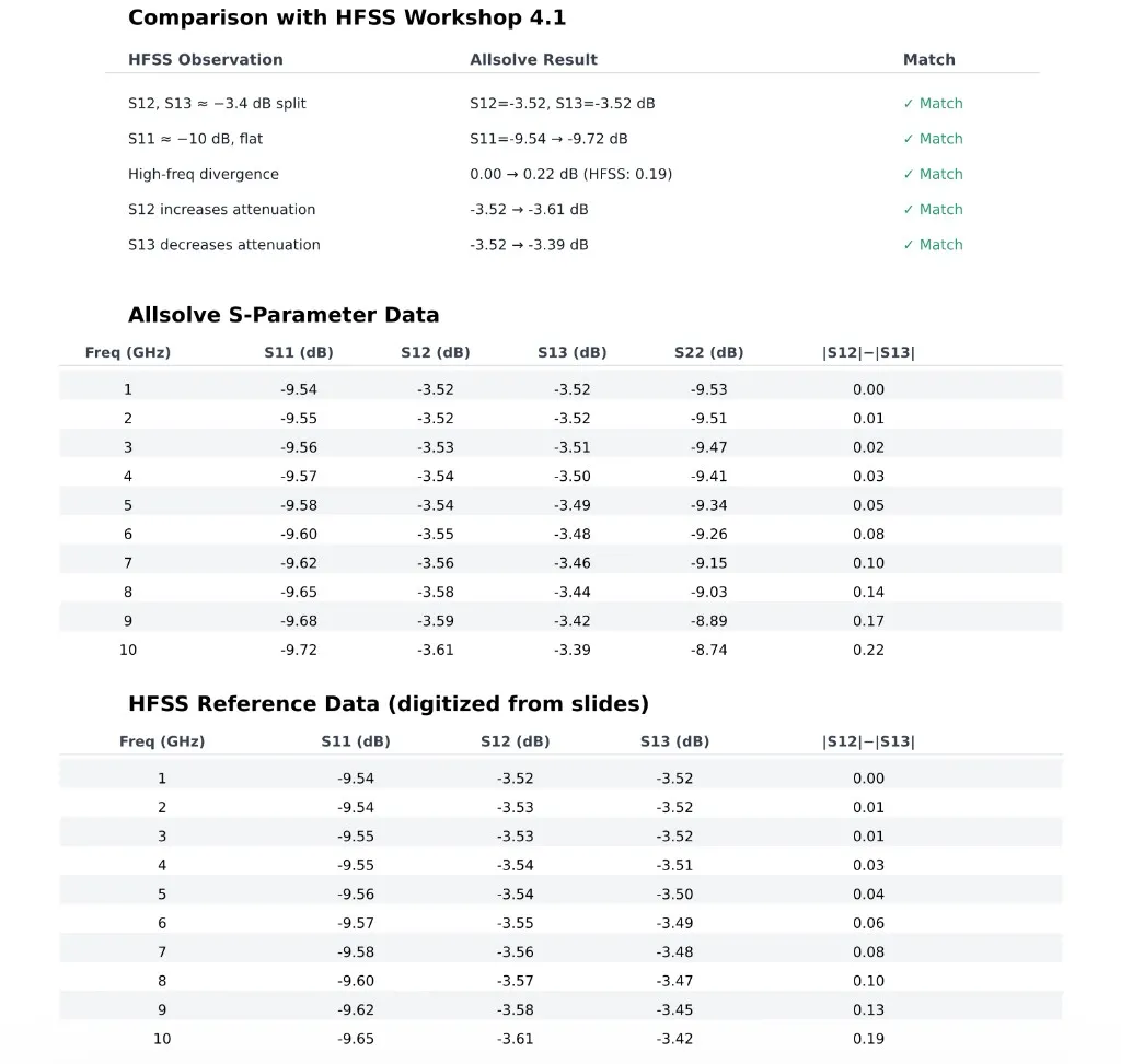
• S11 (reflection): approximately −9.5 dB, nearly flat across the band.
• S12 (branch transmission): approximately −3.5 dB at 1 GHz, decreasing slightly at higher frequencies.
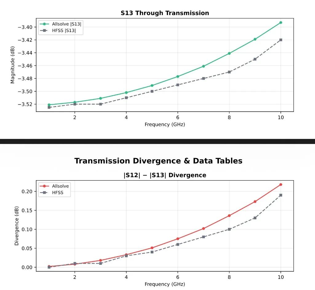
• S13 (through transmission): approximately −3.5 dB at 1 GHz, increasing slightly at higher frequencies.

Power split at high frequency

At low frequencies the junction is electrically small and power divides nearly equally between the branch and through arms. As frequency increases, the straight-through path (port 3) carries slightly more power because the 90-degree bend into the branch creates a small impedance discontinuity. The divergence between S12 and S13 reaches approximately 0.2 dB at 10 GHz.

Results comparison

See the following plots for results comparison with ANSYS HFSS².

S11 reflection and S12 branch transmission

S13 through transmission and divergence between S12 and S13

S-parameter data

References

1. ANSYS, Inc., “HFSS Getting Started — Workshop 4.1: Coax Tee S-Parameters and Fields,” Release 2020 R2. ↩

2. Coaxial Tee S-Parameter Comparison Report, Allsolve simulation vs. ANSYS HFSS Getting Started Workshop 4.1. ↩