Piezocomposite array with backing and matching

What you’ll learn

• How to build a 5×5 piezocomposite array with backing, matching, and water load layers using box geometry, grid, and difference operations.
• How to define custom materials (backing, polymer filler, matching layer) and assign them alongside library materials.
• How to set up transient acoustic–elastic–electrostatic coupled physics with Box PML, proportional damping, viscous damping, and array electrode addressing.
• How to add a custom simulation script with Kirchhoff-Helmholtz beam pattern extraction and FFT post-processing for impedance and transmit sensitivity.

Prerequisites: complete the Piezocomposite transducer tutorial first. It covers the basic geometry, piezoelectricity coupling, and Lump V/Q excitation workflow.

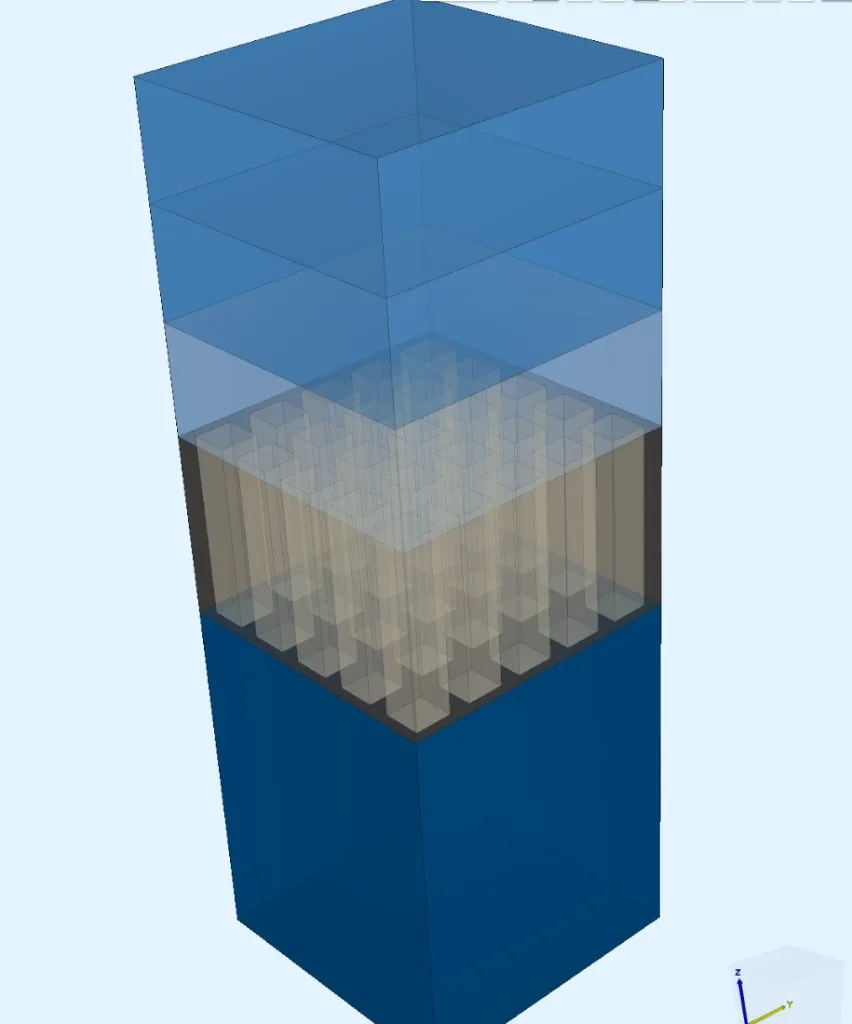
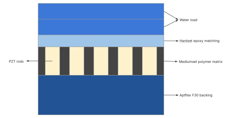
This tutorial models a 5×5 piezocomposite transducer array with backing and matching layers. The centre element is driven with a voltage wavelet, and the simulation produces:

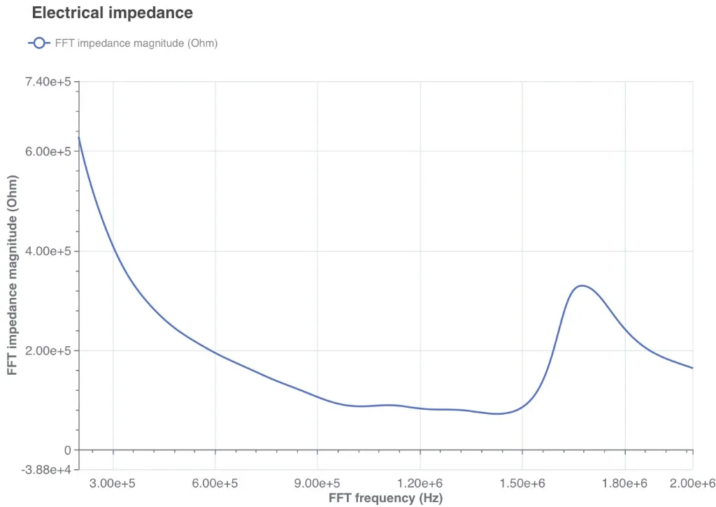
• Electrical impedance Z(f) via FFT
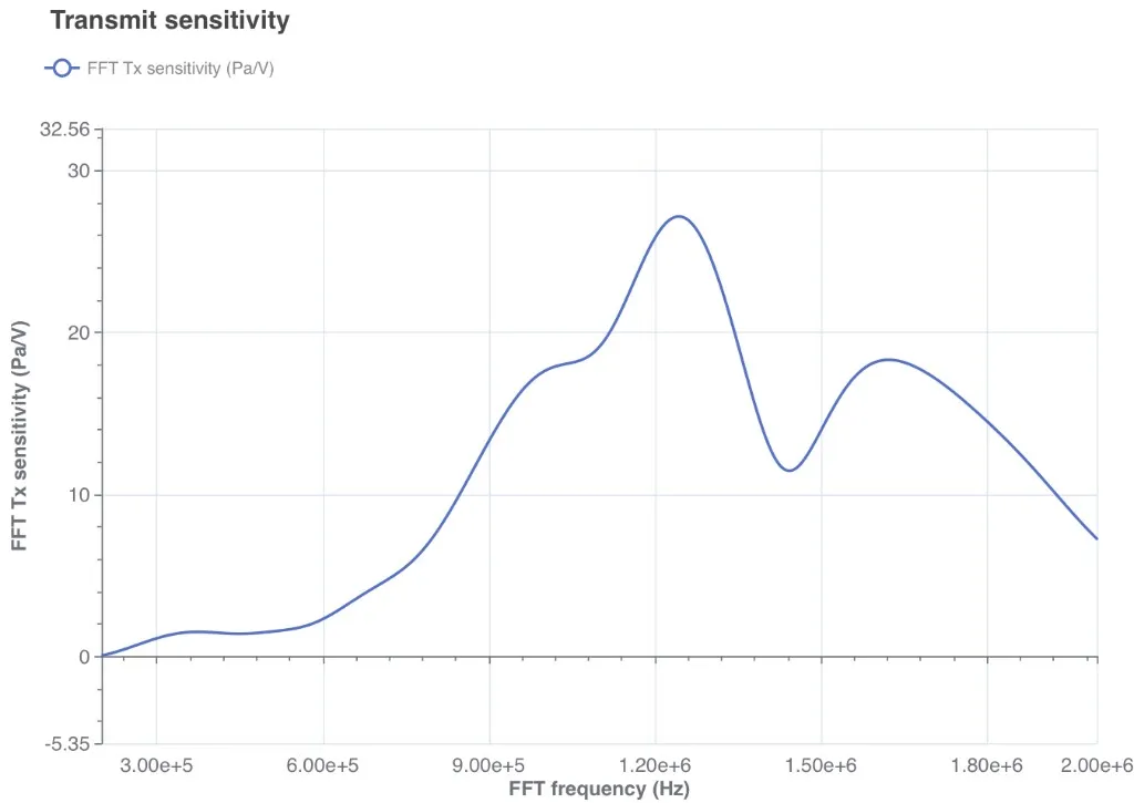
• Front-face and far-field transmit sensitivity (Pa/V)
• Beam pattern via Kirchhoff-Helmholtz extrapolation

Demo project: 1-3 Piezocomposite array

Simulation setup guide

Step 1 — Variables

Create a new project and start without geometry. Open the Common sidebar, Definitions tab, and import the following variables via Import CSV:

Name	Expression	Description
freq	1e6	Centre frequency (Hz)
pitch	0.254e-3	Element pitch (m)
kerf	0.028e-3	Kerf width (m)
pillar	pitch-kerf	Pillar width (m)
array_n	5	Number of pillars per side
array_w	array_n*pitch	Array lateral extent (m)
thk_back	1.5e-3	Backing thickness (m)
thk_comp	0.45e-3	Composite (PZT + kerf) thickness (m)
thk_match	0.35e-3	Matching layer thickness (m)
thk_load	1.5e-3	Water load thickness (m)
ppc	25	Time-steps per cycle
ncycles	10	Number of cycles
mesh_freq	1e6	Mesh sizing frequency (Hz)
q_pzt	50	PZT mechanical Q factor
extr_radius	50e-3	Beam pattern extrapolation radius (m)
extr_angle_step	0.5	Beam pattern angular step (degrees)

You can import the variables as a CSV file:

Name,Expression,Description
freq,1e6,Centre frequency (Hz)
pitch,0.254e-3,Element pitch (m)
kerf,0.028e-3,Kerf width (m)
pillar,pitch-kerf,Pillar width (m)
array_n,5,Number of pillars per side
array_w,array_n*pitch,Array lateral extent (m)
thk_back,1.5e-3,Backing thickness (m)
thk_comp,0.45e-3,Composite (PZT + kerf) thickness (m)
thk_match,0.35e-3,Matching layer thickness (m)
thk_load,1.5e-3,Water load thickness (m)
ppc,25,Time-steps per cycle
ncycles,10,Number of cycles
mesh_freq,1e6,Mesh sizing frequency (Hz)
q_pzt,50,PZT mechanical Q factor
extr_radius,50e-3,Beam pattern extrapolation radius (m)
extr_angle_step,0.5,Beam pattern angular step (degrees)

Step 2 — Geometry

Go to the Geometry section. The model consists of box layers for backing, composite (PZT + polymer), matching, and water. The 5×5 grid of PZT rods is created via grid and difference.

2.1 — Backing box

Add a Box with Alignment = Corner:

Setting	Value
Name	Backing
Corner point (X, Y, Z)	0, 0, 0
Size (X, Y, Z)	array_w, array_w, thk_back

2.2 — Polymer box

Copy the backing box and change:

Setting	Value
Name	Polymer
Corner Z	thk_back
Size Z	thk_comp

2.3 — First PZT rod

Add a Box with Alignment = Corner:

Setting	Value
Name	PZT_1_1
Corner point (X, Y, Z)	kerf/2, kerf/2, thk_back
Size (X, Y, Z)	pillar, pillar, thk_comp

2.4 — Grid the PZT rods

Add a Grid operation:

Setting	Value
Name	PZT
Target	PZT_1_1
Translation (X, Y, Z)	pitch, pitch, 0
Grid size (X, Y, Z)	array_n, array_n, 1

This produces 25 PZT pillars in a 5×5 pattern.

2.5 — Difference (polymer minus rods)

Add a Difference operation:

Setting	Value
Name	Difference
Set 1	Polymer
Set 2	PZT (all rod volumes)
Delete	Unchecked

This takes the rods out of the polymer slab volume, leaving only the kerf filler.

2.6 — Matching layer

Copy the polymer box and change:

Setting	Value
Name	Matching
Corner Z	thk_back + thk_comp
Size Z	thk_match

2.7 — Water load (inside)

Copy the polymer box and change:

Setting	Value
Name	Load
Corner Z	thk_back + thk_comp + thk_match
Size Z	thk_load/2

2.8 — Water load (outside)

Copy and change:

Setting	Value
Name	Load outside
Corner Z	thk_back + thk_comp + thk_match + thk_load/2
Size Z	thk_load/2

The water is split at the midplane to define the Kirchhoff-Helmholtz extrapolation surface between the two volumes.

Select Confirm model changes (Fragment all).

Step 3 — Material regions

In the Common sidebar, Definitions tab:

1. Under Regions, use Mass rule create:

   • Attribute: name
   • Entity type: Volume
   • Select the named geometry volumes from the list.

2. Add a Computed region named Water (Volume, Union):

   • Regions: Load, Load outside

Step 4 — Materials

Go to the Physics section and assign materials:

Library materials

Material	Target region
PZT	PZT (all 25 rods)
Water	Water

Custom materials

Create custom materials for matching, polymer, and backing, with density and Elasticity matrix properties. Set the elasticity matrix type to Pressure and shear wave velocities:

Material	Target	Density (kg/m³)	Pressure velocity (m/s)	Shear velocity (m/s)
Matching	Matching	1150	3000	1200
Polymer	Polymer	1100	2800	1110
Backing	Backing	650	2500	1000

Material library

If you use similar materials often, it is helpful to add them to your library for reuse across projects.

Step 5 — Physics regions

Create the following regions in the Common sidebar, Definitions tab:

PML regions

Region	Type	Method	Selection
array_acoustic_pml	Surface	Manual pick	All outer surfaces of Load outside (9 surfaces total — top + 4 + 4 laterals of the water load)
array_elastic_pml	Surface	Manual pick	All outer surfaces of the solid domain (13 surfaces total — backing bottom + 4 lateral backing + 4 lateral composite + 4 lateral matching)

Electrode regions

Region	Type	Method	Selection
array_drive_3_3	Surface	Manual pick	Z-direction bottom surface of the centre-most PZT rod (row 3, column 3)
array_ground	Surface	Rule selector → bounding box → pick similar	Top surfaces of all 25 PZT rods

Bounding box pick similar

Click the top surface of a corner PZT rod and select the opposite corner rod’s top surface. The bounding box with “pick similar” captures all 25 rod top surfaces at once.

Region	Type	Method	Selection
array_bottom	Surface	Rule selector → bounding box → pick similar	Bottom surfaces of all 25 PZT rods
array_passive_bottom	Computed, Surface	Difference	array_bottom minus array_drive_3_3

Other regions

Region	Type	Method	Selection
beam_extr_plane_v2	Surface	Manual pick	Interface surface between Load and Load outside
array_front_face	Surface	Manual pick	Z-direction top surface of Matching
Elastic	Computed, Volume	Union	All solid volume regions (Backing, Polymer, PZT, Matching)

Step 6 — Physics

In the Physics section, add three physics modules to a new physics set:

Physics	Target region
Acoustic waves	Water
Elastic waves	Elastic
Electrostatics	PZT

Then add the interactions:

Acoustic waves interactions

Interaction	Target / Settings
Acoustic structure	Couple with: Elastic waves
Perfectly Matched Layer	Target: array_acoustic_pml, Type: Box PML

Elastic waves interactions

Interaction	Target / Settings
Perfectly Matched Layer	Target: array_elastic_pml, Type: Box PML
Proportional damping	Rename: PZT damping (Q=50), Target: PZT, Alpha: qtoalpha(freq, q_pzt), Beta: qtobeta(freq, q_pzt)
Viscous damping — Matching	Target: Matching, set damping from material properties
Viscous damping — Polymer	Target: Polymer, set damping from material properties
Viscous damping — Backing	Target: Backing, set damping from material properties

Damping values

The PZT proportional damping uses the built-in qtoalpha and qtobeta helper functions. For viscous damping on backing, polymer, and matching, set the damping in the material properties panel. Refer to the Piezocomposite 2D example project on how to set this up through UI.

Electrostatics interactions

Interaction	Target / Settings
Lump V/Q	Rename: Drive, Target: array_drive_3_3, Voltage: wavelet(freq, 1.2)
Constraint	Name: Ground, Target: array_ground, Value: 0
Piezoelectricity (Elastic waves)	Target: PZT
Constraint	Name: Passive bottom electrodes, Target: array_passive_bottom, Value: 0

Step 7 — Mesh

In the Simulations section, create a new mesh:

Setting	Value
Name	5x5 array mesh
Mesh element size	Absolute
Max size	1000/mesh_freq/6
Node type	4 CPU, 64 GB

The max size expression gives 6 elements per wavelength at the mesh frequency (1 MHz in water). The larger node speeds meshing to a few seconds.

Step 8 — Simulation settings

Create a new simulation:

Setting	Value
Name	Transient 5x5 beam pattern + FFT
Description	Centre-element beam-pattern transient with electrical impedance and front-face transmit sensitivity FFT outputs for UI plotting.
Analysis type	Transient
Timestep algorithm	Generalized alpha
Start time	0
End time	ncycles/freq
Timestep size	1/freq/ppc
Target frequency	freq

Select the mesh, then use Runtime → Estimate node count to verify resource requirements.

Save the simulation settings.

Value outputs

Add a custom value output:

Name	Output expression
V_drive	lump.V

Step 9 — Script customization

Open the simulation script editor. Two custom sections are required:

9.1 — Extrapolation helper fields

Insert a custom section after the fields are created (at row 67):

# Extrapolation helper fields on the inside water volume
dtp = qs.field("h1")
dtp.setorder(reg.load, 2)
ntp = qs.field("h1")
ntp.setorder(reg.load, 2)

9.2 — Custom time loop and post-processing

Insert a custom section after the formulations are created (at row 118). Disable the autogenerated SOLVE section and add this code:

# Custom time loop and far-field extrapolation
import math
import numpy as np

qs.universe.setmumpsicntl(14, 200)

var.step_index = 0.0
var.start_time = 0.0
var.time_step = 1.0 / expr.freq / expr.ppc
var.end_time = expr.ncycles / expr.freq - 1e-08 * var.time_step

timestepper = qs.genalpha(form, qs.vec(form), qs.vec(form))
timestepper.settolerance(1e-05)
timestepper.setrelaxationfactor(-1)
qs.settime(var.start_time)

extr_times = [var.start_time]
extr_pdtpntp = [[fld.p.copy(), dtp.copy(), ntp]]

voltage_history = []
current_history = []
front_pressure_history = []

while qs.gettime() < var.end_time:
    timestepper.allnext(
        relrestol=1e-06,
        maxnumit=1000,
        timestep=var.time_step,
        maxnumnlit=1000,
    )

    dtp.setvalue(reg.beam_extr_plane_v2, qs.dt(fld.p))
    ntp = form.allneumann(reg.beam_extr_plane_v2, reg.load, fld.p)
    extr_times.append(qs.gettime())
    extr_pdtpntp.append([fld.p.copy(), dtp.copy(), ntp])

    voltage = qs.evaluate(port.lump.V)[0]
    charge = qs.evaluate(port.lump.Q)[0]
    current = qs.evaluate(qs.dt(port.lump.Q))[0]
    front_pressure = qs.allaverage(reg.array_front_face, fld.p, 3)

    voltage_history.append(voltage)
    current_history.append(current)
    front_pressure_history.append(front_pressure)

    qs.setoutputvalue("V_drive", voltage, qs.gettime())
    qs.setoutputvalue("Q_drive", charge, qs.gettime())
    qs.setoutputvalue("I_drive", current, qs.gettime())
    qs.setoutputvalue("p_avg_front", front_pressure, qs.gettime())
    if int(var.step_index) % 10 == 0:
        qs.setoutputfield(
            "Z Displacement Field",
            reg.elastic,
            qs.compz(fld.u),
            2,
            qs.gettime(),
        )
    var.step_index += 1

9.3 — FFT post-processing

Continuing in the same custom section, after the time loop:

# --- Transient FFT impedance and transmit sensitivity ---
sample_count = len(voltage_history)
window = np.ones(sample_count)
taper_start = sample_count // 2
taper_count = sample_count - taper_start
window[taper_start:] = 0.5 * (
    1.0 + np.cos(np.pi * np.arange(taper_count) / taper_count)
)

fft_count = sample_count * 20
frequency = np.fft.rfftfreq(fft_count, d=var.time_step)
voltage_fft = np.fft.rfft(np.asarray(voltage_history) * window, fft_count)
current_fft = np.fft.rfft(np.asarray(current_history) * window, fft_count)
pressure_fft = np.fft.rfft(
    np.asarray(front_pressure_history) * window,
    fft_count,
)

current_floor = max(np.max(np.abs(current_fft)) * 1e-12, 1e-30)
voltage_floor = max(np.max(np.abs(voltage_fft)) * 1e-12, 1e-30)
safe_current = np.where(
    np.abs(current_fft) > current_floor,
    current_fft,
    current_floor + 0j,
)
safe_voltage = np.where(
    np.abs(voltage_fft) > voltage_floor,
    voltage_fft,
    voltage_floor + 0j,
)

impedance = voltage_fft / safe_current
tx_sensitivity = np.abs(pressure_fft / safe_voltage)
frequency_out = np.linspace(0.2e6, 2.0e6, 361)
impedance_magnitude = np.interp(
    frequency_out, frequency, np.abs(impedance),
)
impedance_phase = np.interp(
    frequency_out, frequency, np.angle(impedance, deg=True),
)
front_tx_out = np.interp(
    frequency_out, frequency, tx_sensitivity,
)

qs.setoutputvalue("FFT frequency (Hz)", frequency_out.tolist())
qs.setoutputvalue(
    "FFT impedance magnitude (Ohm)", impedance_magnitude.tolist(),
)
qs.setoutputvalue(
    "FFT impedance phase (deg)", impedance_phase.tolist(),
)
qs.setoutputvalue(
    "FFT front-average Tx sensitivity (Pa/V)", front_tx_out.tolist(),
)

9.4 — Beam pattern extraction

Continuing in the same custom section:

# --- Beam pattern via Kirchhoff-Helmholtz extrapolation ---
c_w = mat.water.c()
rho_w = mat.water.rho()
radius = expr.extr_radius
angle_step_deg = expr.extr_angle_step
z_front = expr.thk_back + expr.thk_comp + expr.thk_match

angles_deg = []
angle = -90.0
while angle <= 90.0 + 1e-9:
    angles_deg.append(angle)
    angle += angle_step_deg

extr_delay = radius / c_w
output_times = [
    time_value + extr_delay - 1.0 / expr.freq
    for time_value in extr_times
]
max_pres = []
pres_on_axis = None

for index, angle_deg in enumerate(angles_deg):
    angle_rad = angle_deg * math.pi / 180.0
    coordinate = [
        expr.array_w / 2 + radius * math.sin(angle_rad),
        expr.array_w / 2,
        z_front + radius * math.cos(angle_rad),
    ]
    pressure = qs.helmholtzkirchhoff(
        form,
        reg.beam_extr_plane_v2,
        reg.load,
        fld.p,
        c_w,
        rho_w,
        coordinate,
        output_times,
        extr_times,
        extr_pdtpntp,
    )
    max_pres.append(max(abs(value) for value in pressure))
    if abs(angle_deg) < 1e-9:
        pres_on_axis = pressure

9.5 — Far-field Tx sensitivity and KPIs

# --- On-axis far-field Tx sensitivity ---
far_pressure = np.asarray(pres_on_axis[1:])
far_pressure = far_pressure[-sample_count:]
far_pressure_fft = np.fft.rfft(far_pressure * window, fft_count)
far_tx_sensitivity = np.abs(far_pressure_fft / safe_voltage)
far_tx_out = np.interp(
    frequency_out, frequency, far_tx_sensitivity,
)

peak_index = int(np.argmax(far_tx_out))
center_frequency = float(frequency_out[peak_index])
maximum_tx = float(far_tx_out[peak_index])
impedance_at_center = float(impedance_magnitude[peak_index])
threshold = maximum_tx / 2.0
lower_candidates = np.where(far_tx_out[:peak_index] < threshold)[0]
upper_candidates = np.where(far_tx_out[peak_index:] < threshold)[0]
lower_frequency = (
    float(frequency_out[lower_candidates[-1]])
    if len(lower_candidates)
    else float(frequency_out[0])
)
upper_frequency = (
    float(frequency_out[peak_index + upper_candidates[0]])
    if len(upper_candidates)
    else float(frequency_out[-1])
)
fractional_bandwidth = (
    (upper_frequency - lower_frequency) / center_frequency
)

qs.setoutputvalue("FFT Tx sensitivity (Pa/V)", far_tx_out.tolist())
qs.setoutputvalue("FFT centre frequency (Hz)", center_frequency)
qs.setoutputvalue("FFT maximum Tx sensitivity (Pa/V)", maximum_tx)
qs.setoutputvalue("FFT impedance at centre (Ohm)", impedance_at_center)
qs.setoutputvalue("FFT lower -6 dB frequency (Hz)", lower_frequency)
qs.setoutputvalue("FFT upper -6 dB frequency (Hz)", upper_frequency)
qs.setoutputvalue("FFT fractional bandwidth", fractional_bandwidth)

qs.setoutputvalue("extr_times_0deg", output_times)
qs.setoutputvalue("extr_pres_0deg", pres_on_axis)
qs.setoutputvalue("angles_deg", angles_deg)
qs.setoutputvalue("max_pres", max_pres)

p_max_global = max(max_pres) if max(max_pres) > 0 else 1e-30
db_pattern = [
    20.0 * math.log10(value / p_max_global) if value > 0 else -100.0
    for value in max_pres
]
qs.setoutputvalue("beam_pattern_dB", db_pattern)
qs.printonrank(0, f"Peak extrapolated pressure: {p_max_global:.4e} Pa")

Step 10 — Run simulation

Save and run the simulation with the following settings:

• Compute: 10 nodes of 2 CPU, 32 GB each.

With these settings, the simulation runs in 10 minutes.

Step 11 — Results and plotting

After the simulation completes, add plots in the Simulations section to visualize outputs:

Plot	X axis	Y axis
Electrical impedance	FFT frequency (Hz)	FFT impedance magnitude (Ohm)
Transmit sensitivity	FFT frequency (Hz)	FFT Tx sensitivity (Pa/V)
Beam pattern	angles_deg	beam_pattern_dB
Extrapolated pressure	extr_times_0deg	extr_pres_0deg

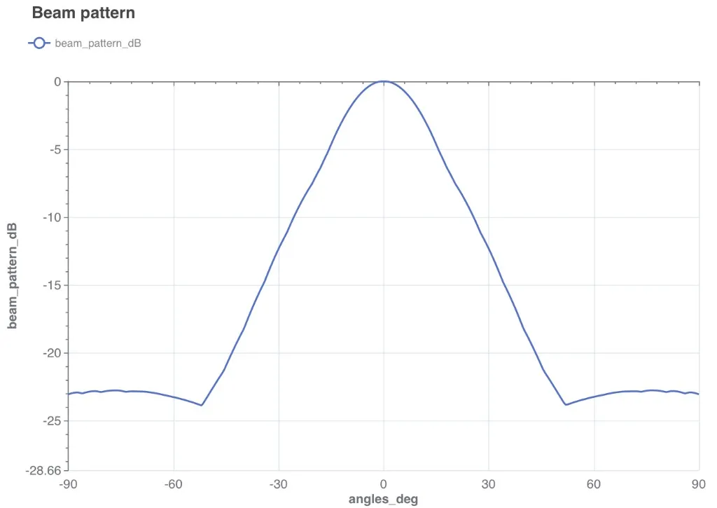
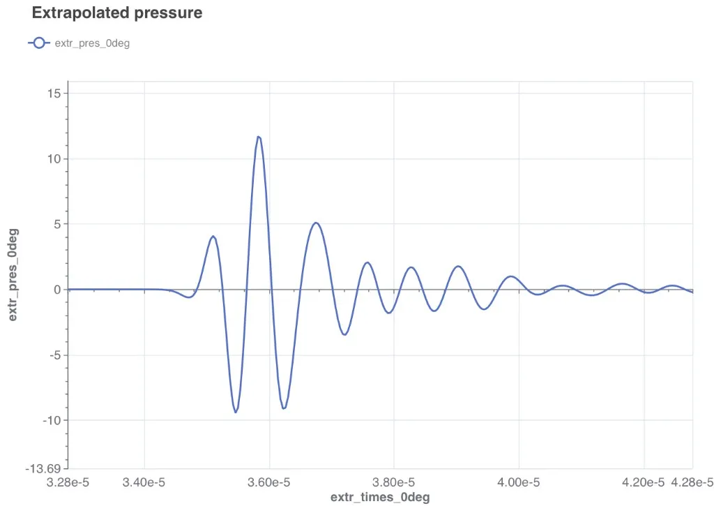
The Z Displacement Field visualization shows the propagating wavefield through the composite stack and into the water load.

Key performance indicators are available as scalar outputs:

KPI	Output name
Centre frequency	FFT centre frequency (Hz)
Maximum Tx sensitivity	FFT maximum Tx sensitivity (Pa/V)
Impedance at centre	FFT impedance at centre (Ohm)
-6 dB fractional bandwidth	FFT fractional bandwidth