PMUT Unit cell - Ultrasound 001
In this step-by-step tutorial, a single PMUT (piezoelectric micromachined ultrasonic transducer) unit cell is modeled and simulated.
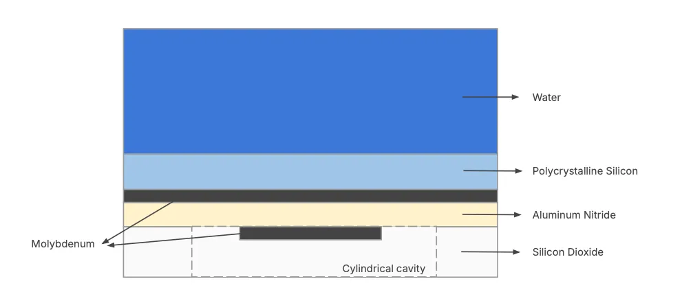
The cell consists of a thin-film stack — silicon dioxide substrate, aluminum nitride piezo layer, molybdenum electrodes, and a polysilicon membrane — coupled to a water load above. Symmetry boundary conditions on the lateral faces represent a periodic array, while an absorbing boundary condition (ABC) truncates the water domain at the top.
Model definition
Section titled “Model definition”The unit cell is built entirely in the Allsolve geometry editor. Each geometry element is given a name, which is then used as a region rule attribute so materials and boundary conditions are easy to set up.
Layer stack
Section titled “Layer stack”| Layer | Geometry name | Material |
|---|---|---|
| Water | vol_water |
Water |
| Polysilicon membrane | vol_poly |
Polycrystalline Silicon |
| Top Mo electrode | vol_mo_top |
Molybdenum |
| AlN piezo layer | vol_aln |
Aluminum Nitride |
| Bottom Mo electrode | vol_mo_bot |
Molybdenum |
| SiO₂ substrate (with cavity) | vol_sio2 |
Silicon Dioxide |
Key variables
Section titled “Key variables”Import all 29 project variables in Step 1. The table below summarizes the most important ones:
| Group | Variables | Role |
|---|---|---|
| Geometry | pitch, cell_d, bot_elec_d, t_sio2, t_aln, t_mo, t_poly |
Stack dimensions |
| Derived geometry | cell_r, bot_elec_r, half_pitch, z_sio2_top, z_aln_top, z_poly_top, z_water_top, eps |
Centers, radii, and region selectors |
| Mesh | lateral_mesh_size, elem_per_wl, lambda_water |
Lateral element size and wavelength meshing in water |
| Simulation | freq, dt, t_end, V_amp, delay, ppc, n_cycles |
Transient settings and drive waveform |
At the default values, the excitation frequency is 12 MHz and the water domain height equals one acoustic wavelength (lambda_water = c_water / freq).
Physics summary
Section titled “Physics summary”| Physics | Target region | Key interactions |
|---|---|---|
| Elastic waves | vol_solid |
Clamp on sur_base; symmetry on sur_sym_x0, sur_sym_xL, sur_sym_y0, sur_sym_yL; Piezoelectricity on vol_aln |
| Acoustic waves | vol_water |
Acoustic structure coupling; Absorbing boundary on sur_water_top |
| Electrostatics | vol_aln |
Constraint (0 V) on sur_top_elec_intf; Lump V/Q drive on sur_bot_elec_intf |
The voltage drive uses V_amp * wavelet(freq, delay).
The function wavelet creates a Ricker wavelet with a given frequency and delay, and is often used as an excitation/load in time-dependent simulations.
Output results
Section titled “Output results”- Drive-port signals: voltage (
drive.V), charge (drive.Q), and current (dt(drive.Q)) - Front-face averages: acoustic pressure, normal displacement, and normal velocity averaged over the radiating surface
- Field outputs: displacement magnitude (
norm(u)) and pressure (p), saved every 25th time step
Step-by-step guide
Section titled “Step-by-step guide”Here you’ll find a detailed step-by-step tutorial on how to build and simulate a PMUT unit cell in Quanscient Allsolve.
Step 1 - Create the project and import variables
Section titled “Step 1 - Create the project and import variables”-
Create a new project and name it
PMUT unit cell. -
Open the Common sidebar, Definitions tab.
-
Import the variables from a CSV file. In the Variables section, use Import CSV and upload a file with the following contents:
Name,Expression,Descriptionfreq,12e6,Centre excitation frequency (Hz)V_amp,1.0,Drive voltage amplitude (V)delay,1.2,Wavelet delay in periods (peak at delay/freq)pitch,60e-6,Inter-cell pitch (m)cell_d,50e-6,Cavity / cell diameter (m)bot_elec_d,25e-6,Bottom electrode diameter (m)t_sio2,2e-6,SiO2 substrate thickness (m)t_aln,1e-6,AlN piezo layer thickness (m)t_mo,200e-9,Molybdenum electrode thickness (m)t_poly,2e-6,Polysilicon elastic layer thickness (m)c_water,1500,Speed of sound in water (m/s)lambda_water,c_water / freq,Acoustic wavelength in water (m)elem_per_wl,6,Mesh elements per wavelength in waterlateral_mesh_size,10e-6,Lateral mesh element size (m)ppc,25,Time-steps per cycledt,1/(freq*ppc),Time-step size (s)n_cycles,10,Number of excitation cycles to simulatet_end,n_cycles/freq,Total simulation time (s)cell_r,cell_d/2,Cell radius (m)bot_elec_r,bot_elec_d/2,Bottom electrode radius (m)half_pitch,pitch/2,Half of inter-cell pitch (m)eps,0.05e-6,Tolerance for bounding-box region selection (m)z_sio2_bot,0,z of SiO2 bottom face (base of stack)z_sio2_top,t_sio2,z of SiO2 top face / AlN bottom facez_aln_bot,z_sio2_top,z of AlN bottom facez_aln_top,z_aln_bot + t_aln,z of AlN top facez_mo_top_top,z_aln_top + t_mo,z of top Mo electrode upper facez_poly_top,z_mo_top_top + t_poly,z of polysilicon top face (front face)z_water_top,z_poly_top + lambda_water,z of water domain top face
Step 2 - Build the geometry
Section titled “Step 2 - Build the geometry”Go to the Geometry section and build the stack from the bottom up. Give each element the Name shown below — these names are used later in region rules and boolean targets.
2.1 — SiO₂ substrate and cavity
Section titled “2.1 — SiO₂ substrate and cavity”-
Add a Box named
sio2_raw:Setting Value Size (X, Y, Z) pitch,pitch,t_sio2Center (X, Y, Z) 0,0,t_sio2/2 -
Add a Cylinder named
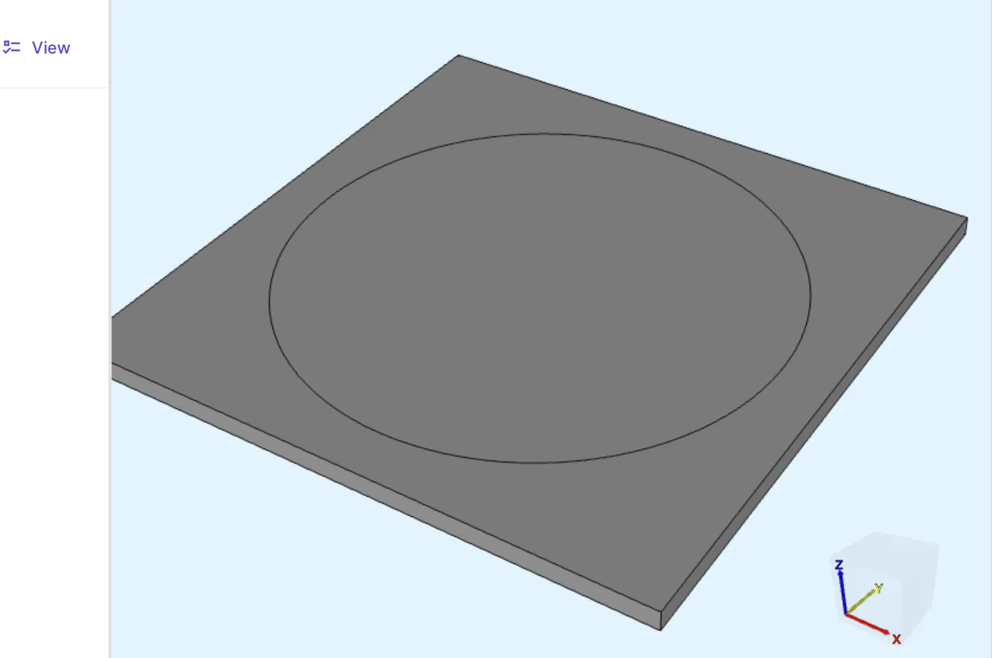
cavity_void:Setting Value Radius cell_rHeight t_sio2Center (X, Y, Z) 0,0,t_sio2/2Build both elements. The substrate block and cavity cutter should look like this:
-
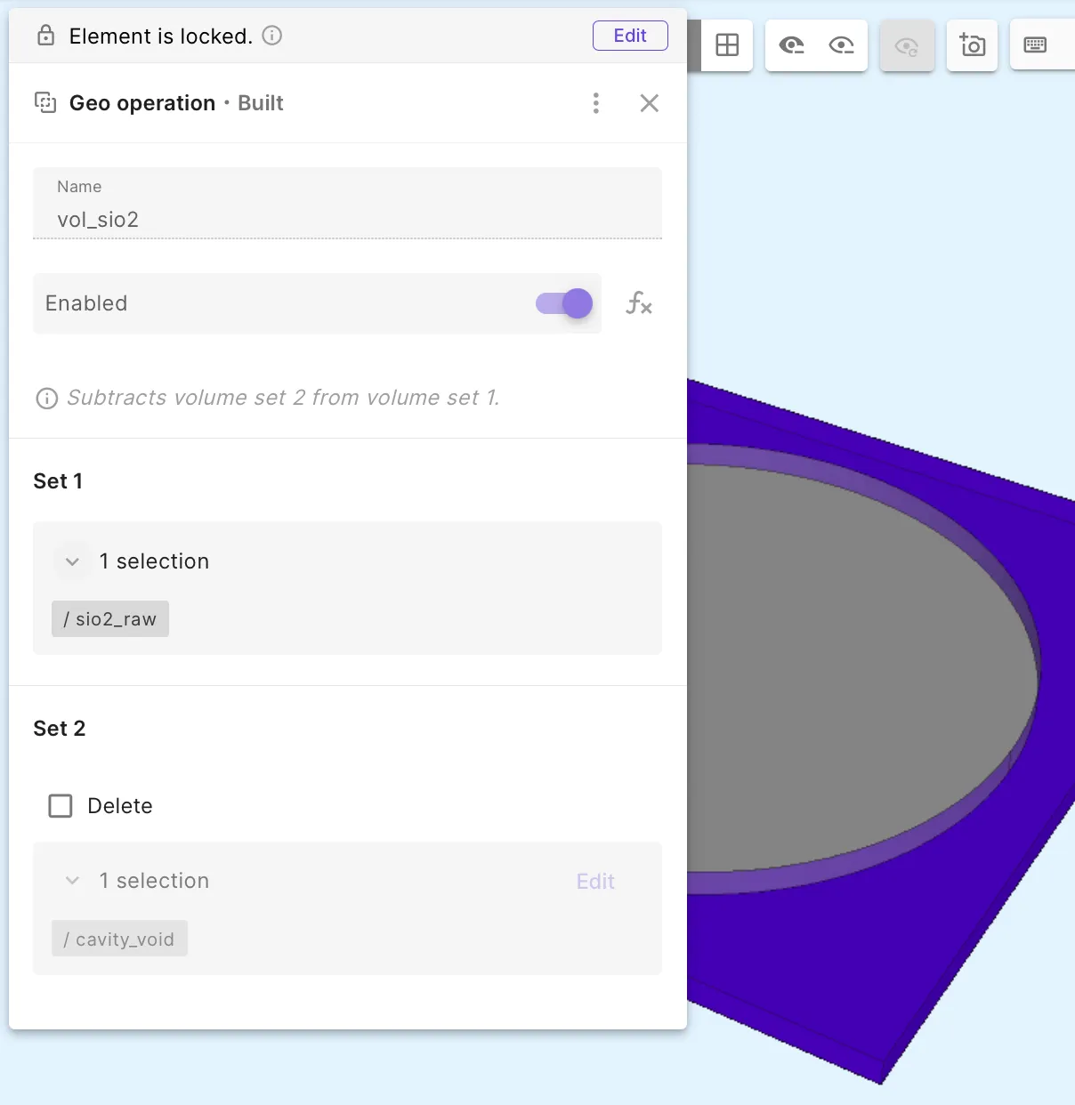
Add a Difference operation named
vol_sio2:Setting Value Set 1 /sio2_rawSet 2 /cavity_voidDelete Unchecked This subtracts the cavity cylinder from the substrate without deleting the cutter volume from the model tree yet.
-
Add a Remove operation named
remove_cavitywith Target/cavity_void.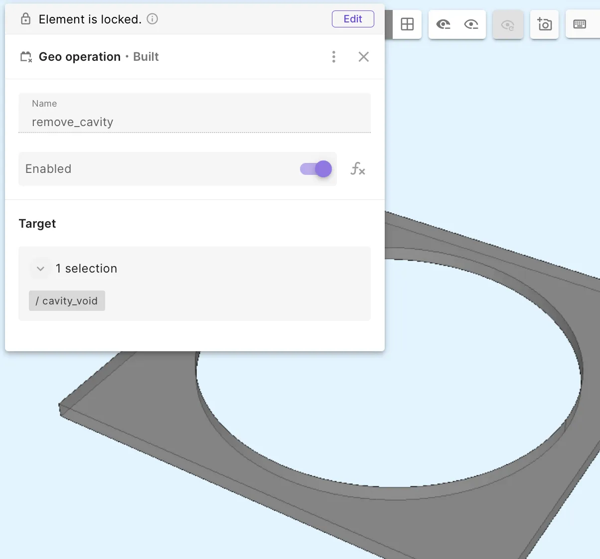
2.2 — Bottom Mo electrode
Section titled “2.2 — Bottom Mo electrode”-
Add a Cylinder named
vol_mo_bot:Setting Value Radius bot_elec_rHeight t_moCenter (X, Y, Z) 0,0,z_aln_bot - t_mo/2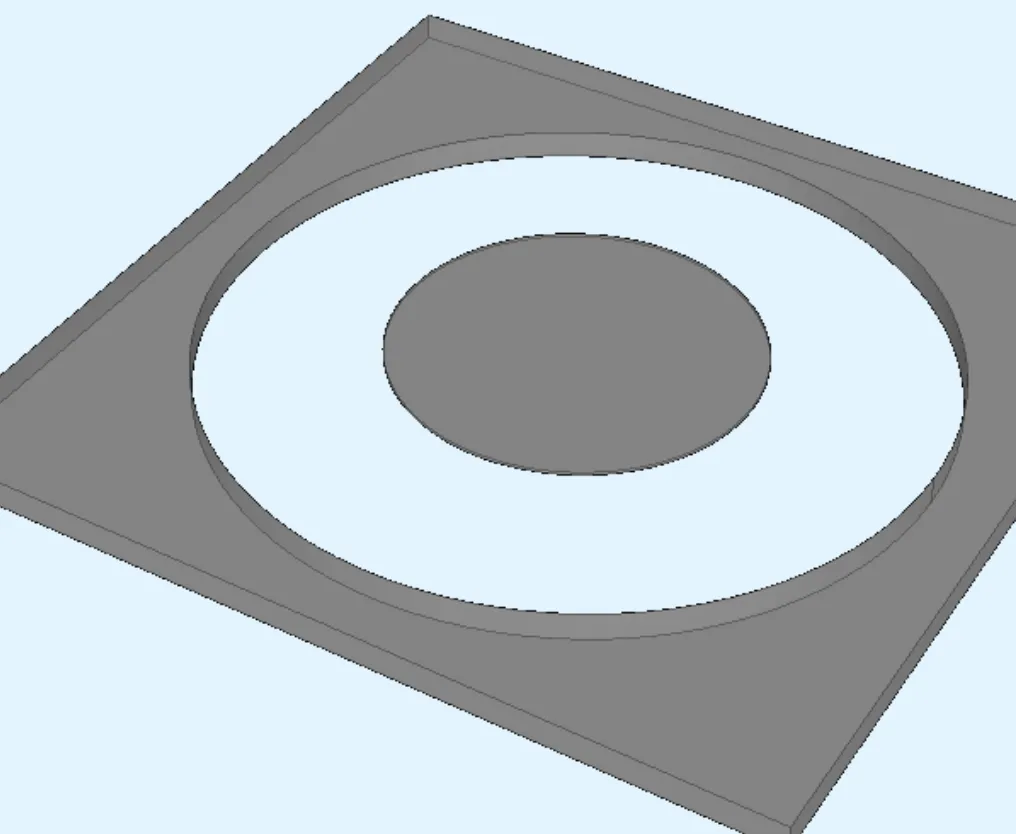
2.3 — Remaining layers
Section titled “2.3 — Remaining layers”Add a Box for each layer:
| Name | Size (X, Y, Z) | Center (X, Y, Z) |
|---|---|---|
vol_aln |
pitch, pitch, t_aln |
0, 0, z_aln_bot + t_aln/2 |
vol_mo_top |
pitch, pitch, t_mo |
0, 0, z_aln_top + t_mo/2 |
vol_poly |
pitch, pitch, t_poly |
0, 0, z_mo_top_top + t_poly/2 |
vol_water |
pitch, pitch, lambda_water |
0, 0, z_poly_top + lambda_water/2 |
Build each element. Your geometry list should contain vol_sio2, vol_mo_bot, vol_aln, vol_mo_top, vol_poly, and vol_water:
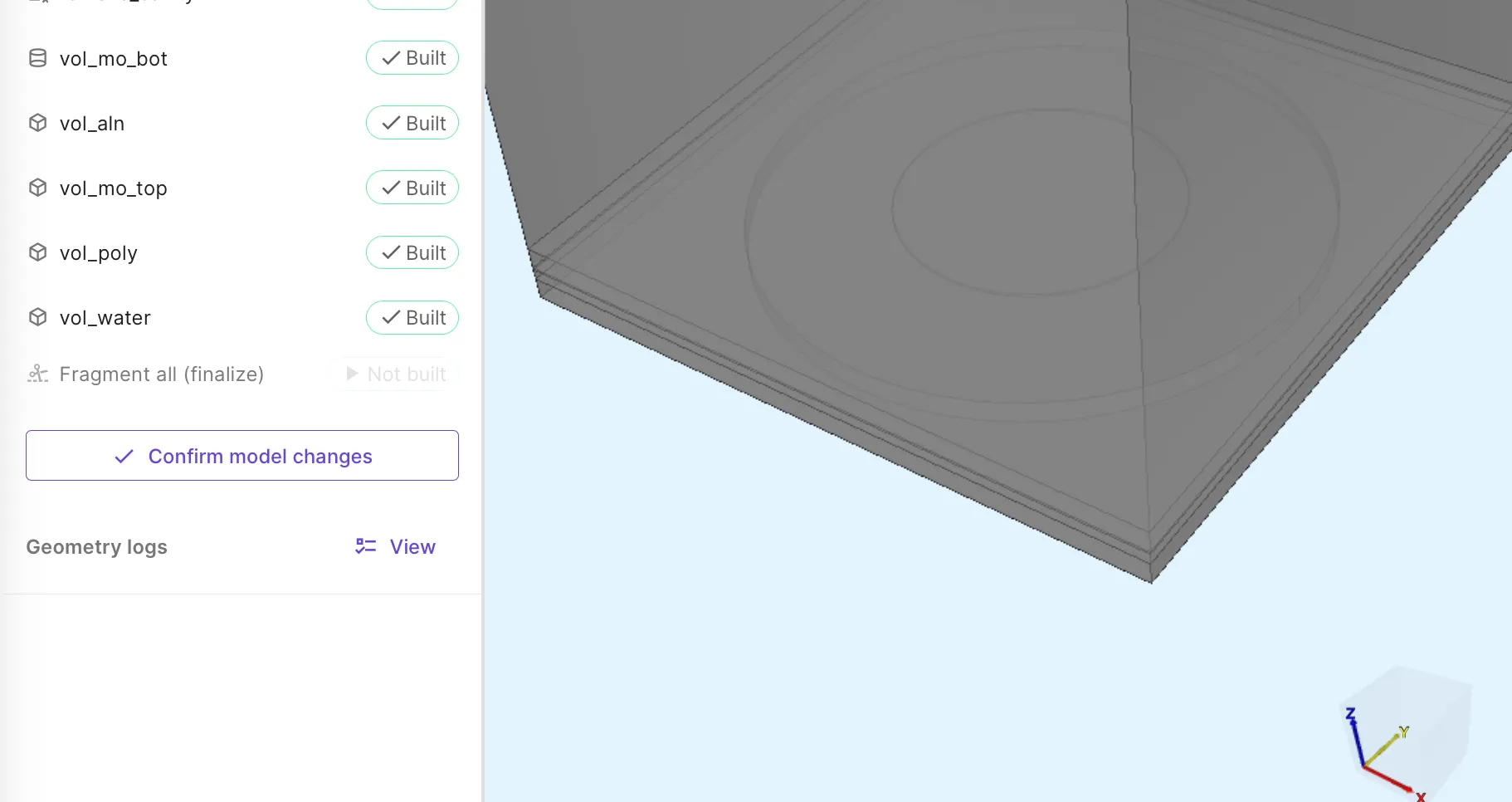
-
Add Fragment all (finalize) and select
Confirm model changes.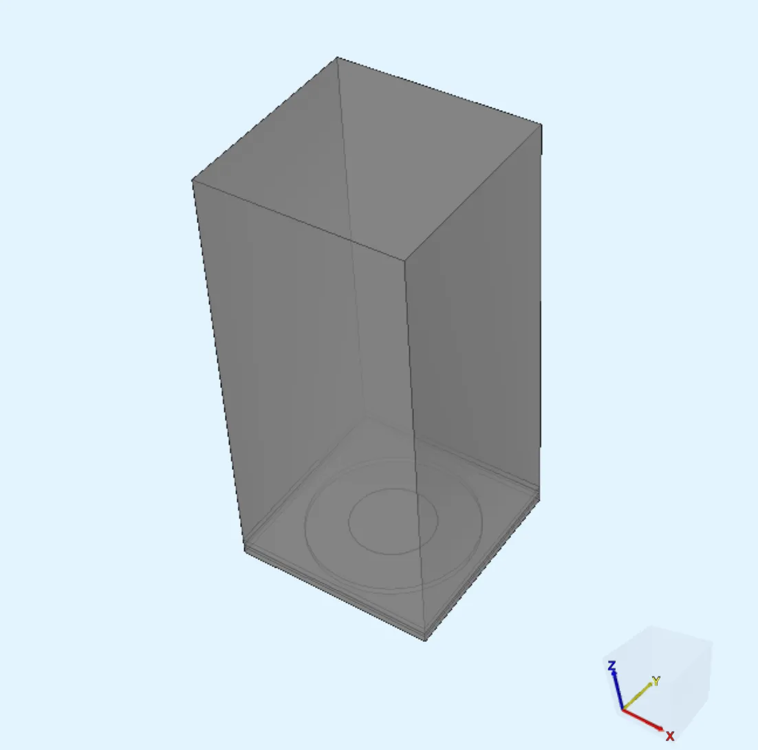
Step 3 - Create material regions
Section titled “Step 3 - Create material regions”Return to the Common sidebar, Definitions tab.
-
Under Regions, use Mass rule create:
- Attribute:
name - Entity type: Volume
This creates one volume region for each named geometry element (
vol_sio2,vol_mo_bot,vol_mo_top,vol_aln,vol_poly,vol_water).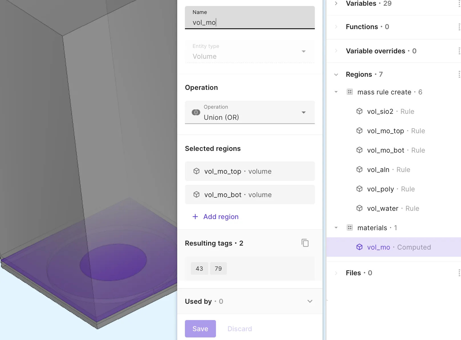
- Attribute:
-
Add a Computed region named
vol_mo:Setting Value Entity type Volume Operation Union (OR) Regions vol_mo_top,vol_mo_bot
Step 4 - Assign materials
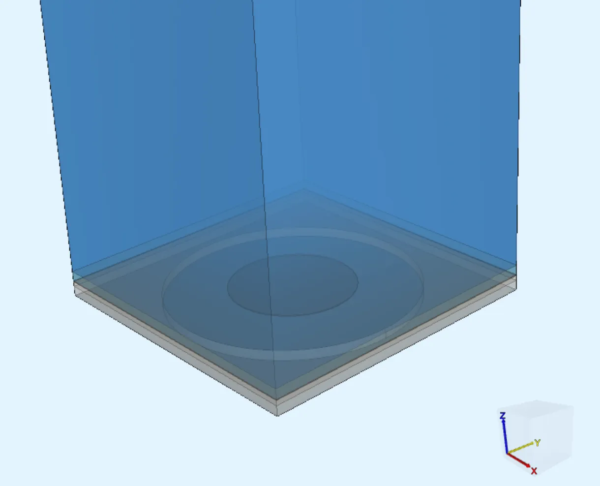
Section titled “Step 4 - Assign materials”Go to the Physics section and assign materials from the global library:
| Material | Target region |
|---|---|
| Silicon Dioxide | vol_sio2 |
| Aluminum Nitride | vol_aln |
| Molybdenum | vol_mo |
| Polycrystalline Silicon | vol_poly |
| Water | vol_water |
Step 5 - Create physics regions
Section titled “Step 5 - Create physics regions”Back in the Common sidebar, define surface and volume regions for boundary conditions.
5.1 - Solid domain
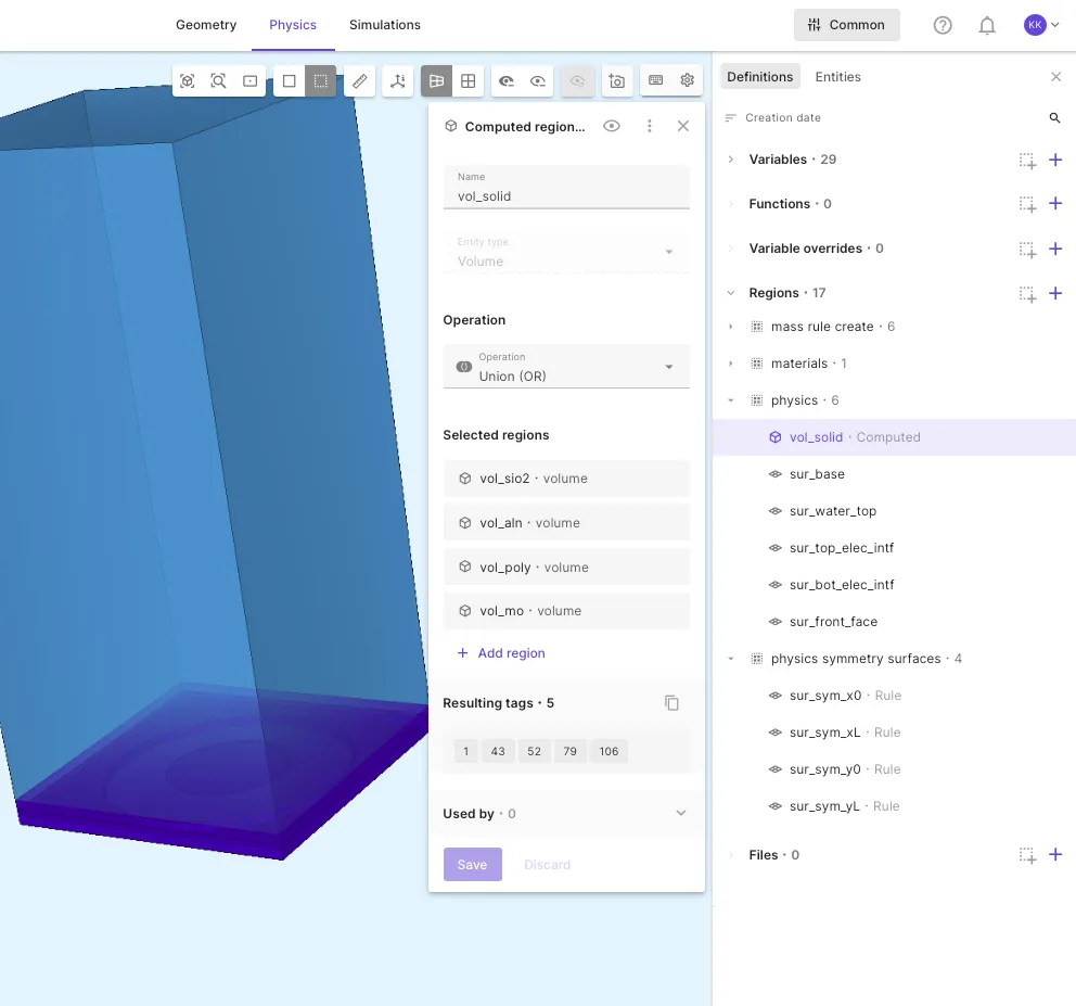
Section titled “5.1 - Solid domain”Add a Computed region named vol_solid (entity type Volume, operation Union):
| Regions to union |
|---|
vol_sio2, vol_aln, vol_poly, vol_mo |
5.2 - Boundary surfaces
Section titled “5.2 - Boundary surfaces”Create Surface regions by picking on the model view:
| Region | Selection hint |
|---|---|
sur_base |
Bottom face of the stack at z = z_sio2_bot (this surface has a circular cut-out due to the cylinder cavity) |
sur_water_top |
Top face of the water box at z = z_water_top |
sur_top_elec_intf |
Interface between the top Mo electrode and the polysilicon layer |
sur_bot_elec_intf |
Top face of the bottom Mo electrode disc |
sur_front_face |
Front face of the unit cell (boundary surface between water and poly-Si) |
5.3 - Symmetry surfaces
Section titled “5.3 - Symmetry surfaces”For the four lateral symmetry faces, use Rule selector with Bounding box and Pick similar:
- Create a surface region named
sur_sym_x0. - Select top-most and bottom-most surfaces in the x0 plane, so that the bounding box includes all 4 solid region surfaces in that plane.
- Repeat for
sur_sym_xL,sur_sym_y0,sur_sym_yL.
Step 6 - Define physics and boundary conditions
Section titled “Step 6 - Define physics and boundary conditions”In the Physics section, add three modules to your physics set: Elastic waves, Acoustic waves, and Electrostatics.
Physics 1 — Elastic waves
Section titled “Physics 1 — Elastic waves”-
Set Elastic waves target to
vol_solid. -
Add a Clamp interaction named
ClampBaseonsur_base.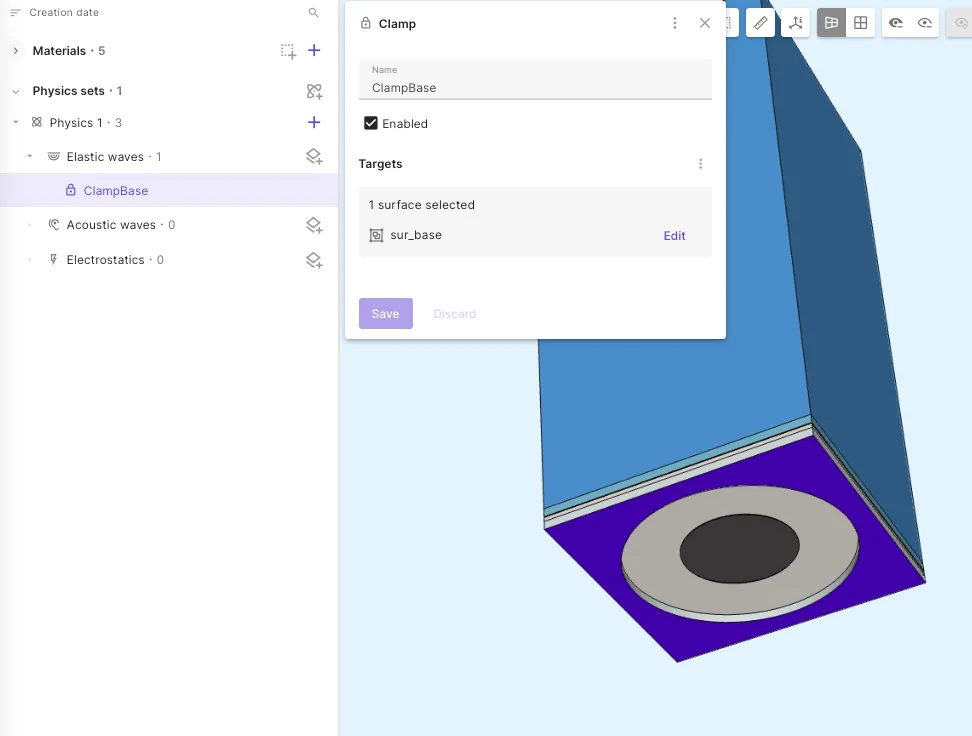
-
Add four Symmetry interactions:
Name Target SymmetryX0sur_sym_x0SymmetryXLsur_sym_xLSymmetryY0sur_sym_y0SymmetryYLsur_sym_yL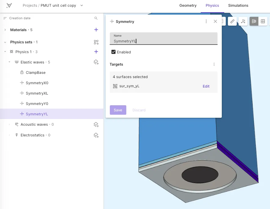
-
Add Piezoelectricity with target
vol_aln.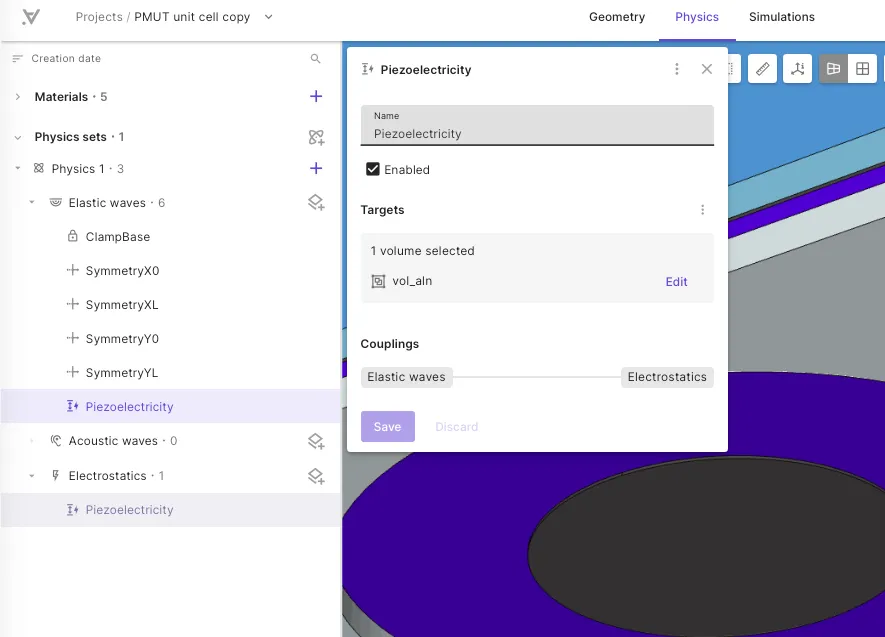
Physics 2 — Acoustic waves
Section titled “Physics 2 — Acoustic waves”-
Set Acoustic waves target to
vol_water. -
Add Acoustic structure (
AW_EW_Coupling) to couple acoustic and elastic domains. -
Add an Absorbing boundary named
WaterTopABConsur_water_top.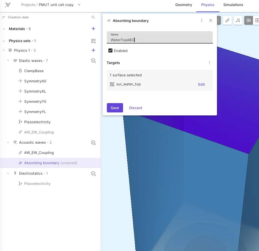
Physics 3 — Electrostatics
Section titled “Physics 3 — Electrostatics”-
Set Electrostatics target to
vol_aln. -
Add a Constraint named
GroundTopElectrodeonsur_top_elec_intfwith Constraint value0.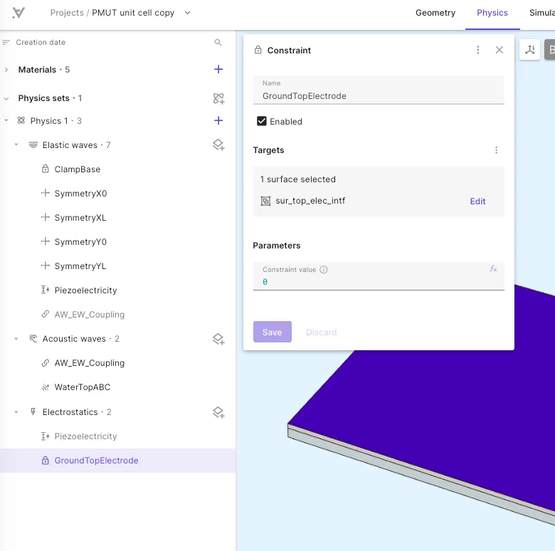
-
Add a Lump V/Q named
DrivePort:Setting Value Namespace driveTarget sur_bot_elec_intfActuation mode Voltage Voltage V_amp * wavelet(freq, delay)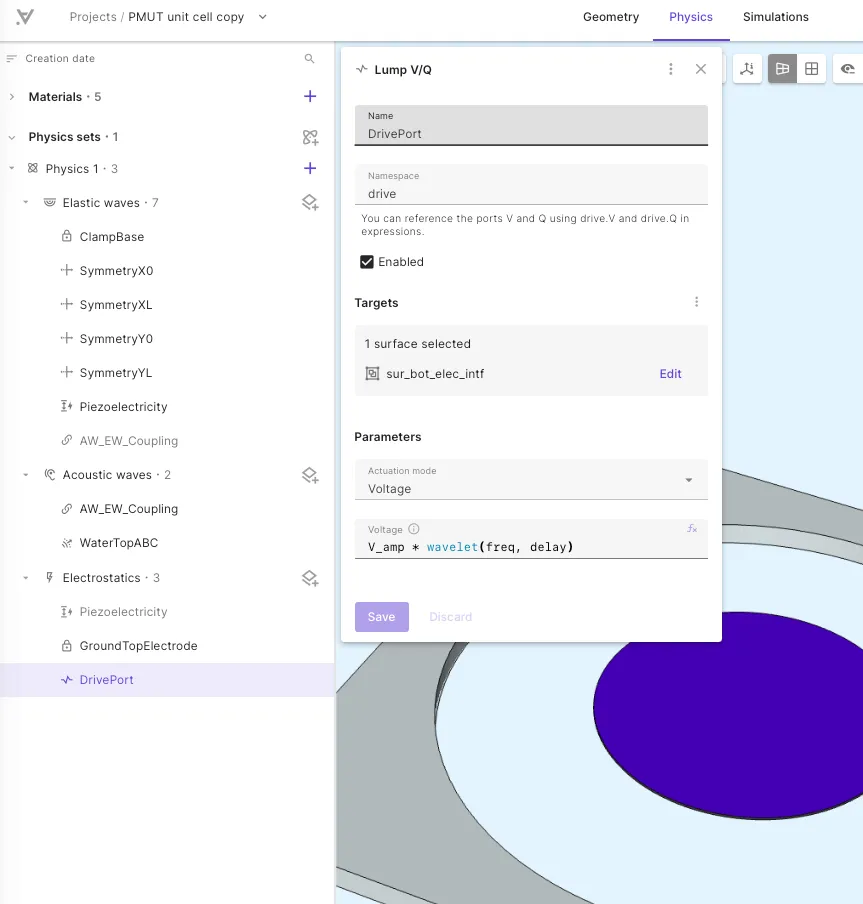
Step 7 - Generate the mesh
Section titled “Step 7 - Generate the mesh”Go to the Simulations section and create a new mesh:
-
Set Autorefine to
Disabled. -
Under Mesh element size, set Max size to
lateral_mesh_sizewith type Absolute. -
Under Runtime, set Node type to
Fast start. -
Under Customizations, add Mesh extrusion → Simple extrusion:
- Target: select all six volumes.
- Sublayers (from top down; water first):
elem_per_wl,1,1,1,1,1.
See Simple extrusion for more on layered extruded meshing.
-
Apply settings and mesh. Check the preview:
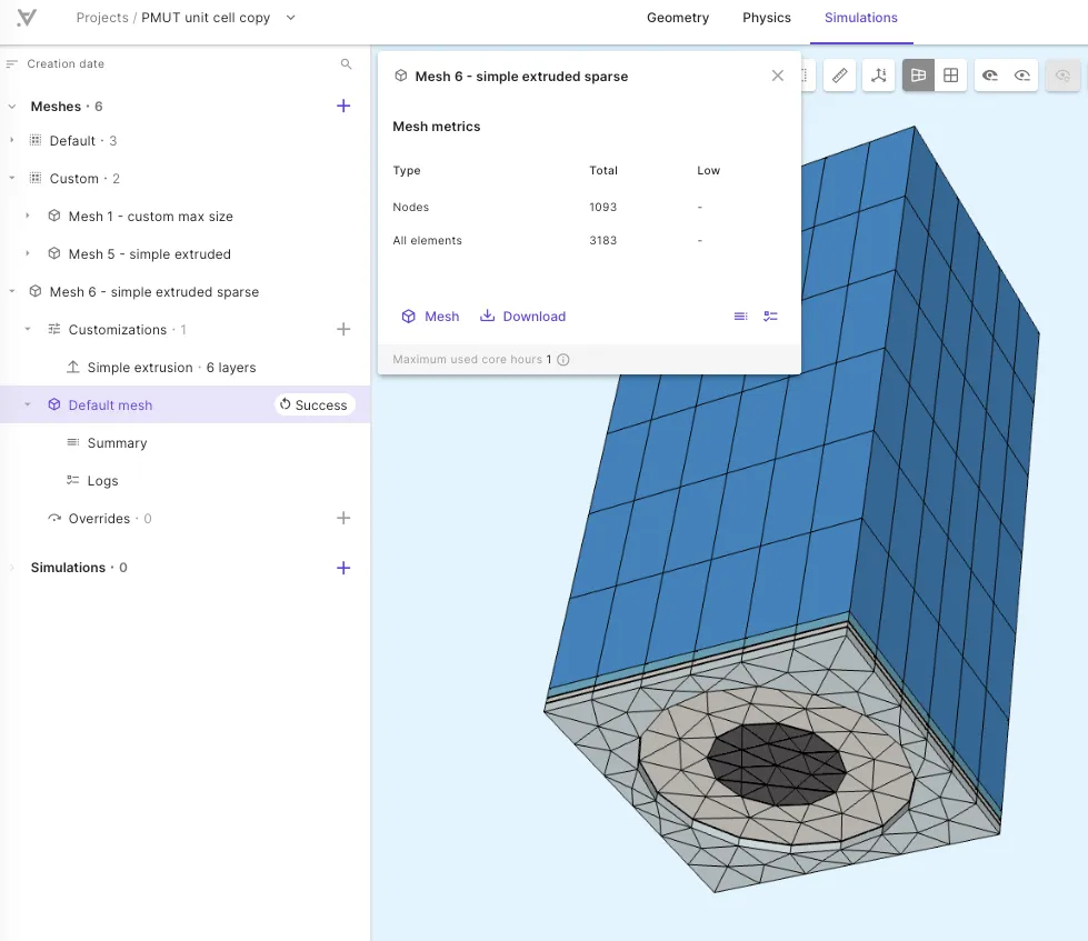
Step 8 - Create the simulation and run
Section titled “Step 8 - Create the simulation and run”-
Create a new simulation named
PMUT Unit Transient. -
Set Analysis type to
Transient. -
Configure Generalized alpha timestepping:
Setting Value Start time 0End time t_endTimestep size dtTarget frequency freq -
Select the extruded mesh.
-
Add Outputs. First, add the drive-port value outputs:
Name Expression V_drivedrive.VQ_drivedrive.QI_drivedt(drive.Q)Then add surface-averaged value outputs on the front face of the unit cell:
Name Expression p_avg_frontaverage(reg.sur_front_face, p, 3)uz_avg_frontaverage(reg.sur_front_face, compz(u), 3)vz_avg_frontaverage(reg.sur_front_face, dt(compz(u)), 3)These track the average acoustic pressure, normal displacement, and normal velocity on the radiating surface.
Finally, add field outputs for visualization. Set the filter to Output every Nth step with an interval of
25on both:Name Expression u_magnorm(u)pressurep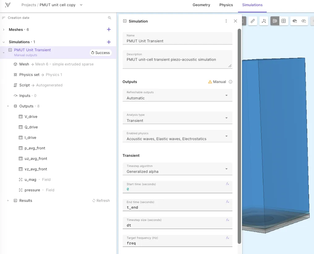
-
Run the simulation.
Step 9 - Plot & visualize results
Section titled “Step 9 - Plot & visualize results”Once the simulation completes, inspect the outputs to verify that the PMUT behaves as expected.
In the Simulations section:
-
Add Plots for the drive-port Voltage, Charge, and Current custom values over time.
-
Add a Visualization for the pressure field
pin the water load (for example with a Slice filter through the cell center). -
Add a Visualization for displacement
uin the solid stack.
Results
Section titled “Results”Drive-port signals
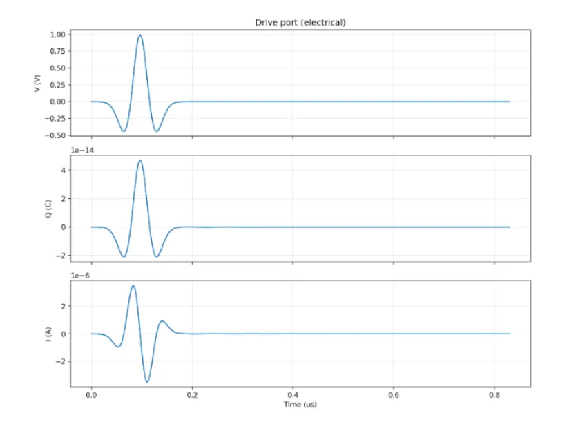
Section titled “Drive-port signals”The drive port plots show the applied Ricker wavelet voltage, the charge accumulated on the bottom electrode, and the resulting current. The wavelet peaks at delay / freq ≈ 100 ns, after which the current decays rapidly — confirming that the excitation is compact in time and well-suited for broadband characterization.
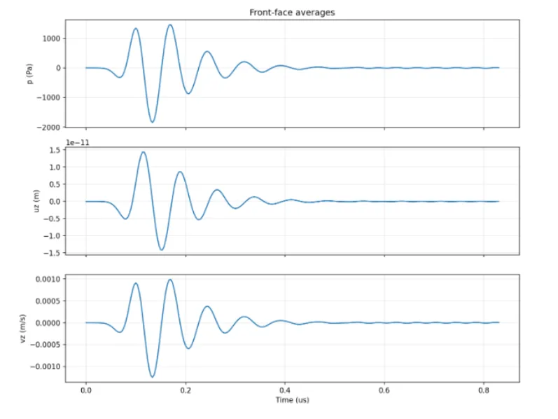
Front-face averages
Section titled “Front-face averages”The surface-averaged pressure, displacement, and velocity on the radiating front face reveal the transducer’s impulse response. After the initial excitation, the membrane rings down over several cycles. The peak pressure reaches approximately 2 kPa and the normal velocity is on the order of 1 mm/s — typical values for a PMUT driven at 1 V.
Frequency-domain performance
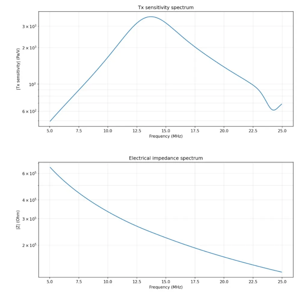
Section titled “Frequency-domain performance”By applying an FFT to the time-domain results, you can extract the transmit sensitivity spectrum (Pa/V) and the electrical impedance spectrum. The sensitivity peaks near 13–14 MHz, indicating the fundamental flexural resonance of the membrane. The impedance curve shows a predominantly capacitive response, as expected for a thin piezoelectric film operating below its thickness-mode resonance.