Simulations overview

What you’ll learn

• Creating simulations: Set up new simulations or copy existing ones.
• Physics sets: Select which physics configuration a simulation solves.
• Analysis types: Choose between static, harmonic, multiharmonic, transient, and eigenmode analysis.
• Solver settings: Select the direct or iterative solver and tune solver parameters.

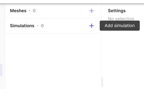
Projects in Quanscient Allsolve can have multiple simulations. Simulations are created and modified in the Simulations section:

The Simulations section in the project top navigation

A new, blank simulation is created by selecting + next to Simulations:

Creating a new simulation with the + button

You can also create a simulation by copying an existing one:

Copying an existing simulation from the context menu

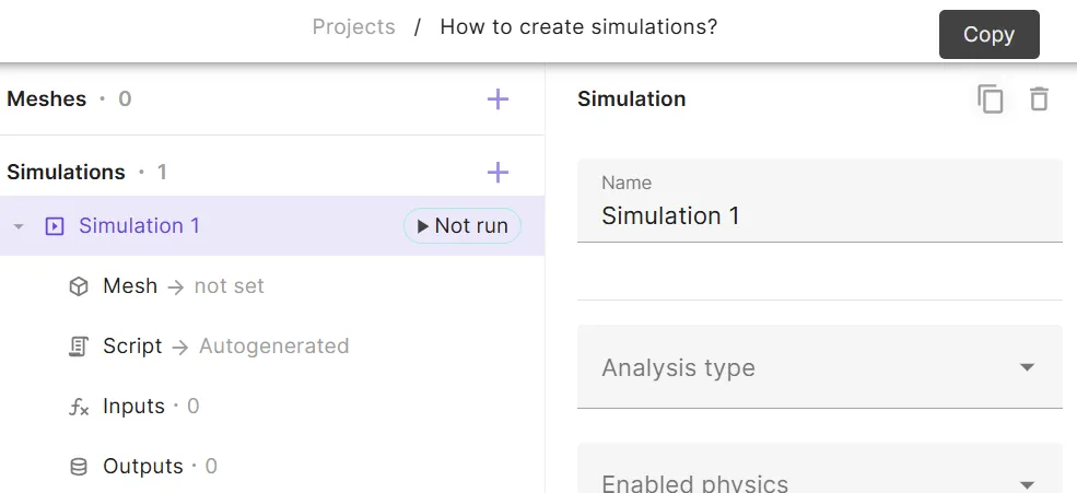
When copying a simulation, all settings are also copied from the original, which is convenient when creating multiple simulations with similar options.

Before running a simulation, configure physics in the Physics section. Physics are grouped into physics sets — each simulation solves one set at a time. See Working with physics for how to create sets, add physics, and define interactions and couplings.

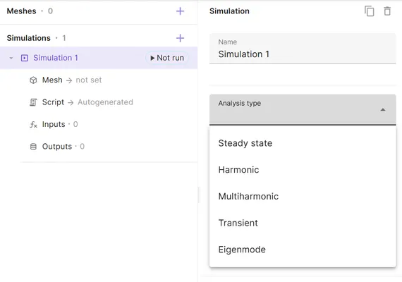
Analysis types

Quanscient Allsolve offers five analysis types:

• Static
  • Time-independent systems
• Harmonic
  • Sinusoidal input
  • For linear problems
• Multiharmonic
  • Input is a combination of multiple sinusoidal frequencies
  • For nonlinear problems
• Transient
  • Time-dependent systems
  • Time-stepping
• Eigenmode
  • Determine the natural frequencies and associated mode shapes of a system

Choosing analysis type

Choosing the right analysis type depends on the nature of the problem at hand. Most analysis types and physics are compatible, but there are exceptions.

The compatibility of analysis types and physics is shown below:

	Static	Harmonic	Multiharmonic	Transient	Eigenmode
Solid Mechanics
Current flow
Acoustic waves	NA
Electrostatics
Electromagnetic waves	NA
Magnetism A
Magnetism φ
Magnetism H
Laminar flow
Heat solid
Heat fluid
Elastic waves	NA
Mesh deformation

NA = Not Applicable

To pick an analysis type, select it in the drop-down list in the simulation settings

Static

Static analysis studies systems where the field variables do not change over time. The partial time derivative term $\partial(\cdot)/\partial t$ in the partial differential equation is assumed zero. You can think of it like a snapshot of a system after all the initial fluctuations have settled.

Static analysis is ideal for problems where the system is stable and the goal is to determine a final equilibrium state.

Harmonic

Harmonic analysis studies systems that respond to a sinusoidal input (e.g., a force or vibration) with a sinusoidal output.

Harmonic analysis is suitable for analyzing systems that experience simple periodic vibrations or oscillations. It helps determine the system’s response at different frequencies. Hence, harmonic simulations are often used with frequency sweeps.

Linearity

The harmonic analysis type is designed for linear problems only.

Multiharmonic

Multiharmonic analysis is an extension of harmonic analysis, and it considers systems where the input is not a single sinusoid but a combination of multiple frequencies.

Multiharmonic analysis suits systems that are excited by multiple frequencies simultaneously.

Nonlinearity

The multiharmonic analysis type is designed for nonlinear problems, as an extension of the linear harmonic analysis type.

Transient

Transient analysis examines how a system evolves over time in response to changing conditions. It calculates the system’s response at various time steps.

Transient analysis is essential for problems where the system’s behavior changes dynamically with time.

Generalized alpha

The Generalized alpha timestepping algorithm takes the following parameters:

Parameter	Description
Start time (seconds)	The simulation start time. Defaults to 0.
End time (seconds)	The simulation end time.
Timestep size (seconds)	The size of each time step. A smaller timestep gives higher temporal resolution but increases the number of steps and total computation time.
Target frequency (Hz)	A convenience parameter that helps size the timestep for wave or oscillation problems. When set, the solver ensures that the timestep is small enough to resolve the specified frequency.

Tip

All transient parameters accept expressions, so you can use variables and functions (e.g. t_end, dt, freq) defined in the common sidebar.

Setting timestep size

When working with wave or oscillation problems, such as ultrasound, it’s a common practice to define timestep size based on frequency.

20 timesteps per period is a good starting point for example, so timestep size = 1/freq/20.

Eigenmode

Eigenmode analysis is used to determine the natural frequencies (eigenfrequencies) and associated mode shapes (eigenmodes) of a system. These are the frequencies and modes at which the system tends to vibrate or oscillate naturally when subjected to an initial disturbance with no other external driving force.

Eigenmode analysis is important for understanding the dynamic characteristics of structures, determining potential resonance risks, and designing systems to avoid excessive vibrations or deformations.

Physics set

Each simulation solves one physics set from your project. In the sidebar, select Physics set under your simulation to choose which set to use:

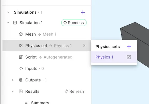
Select next to a set to open it in the Physics section for editing. Create and configure sets there (see Working with physics).

A project can contain multiple physics sets — for example, one set with only Solid mechanics and another with Elastic waves, Acoustic waves, and Electrostatics for a piezoelectric transducer. To compare different physics configurations, create separate sets and assign each to its own simulation.

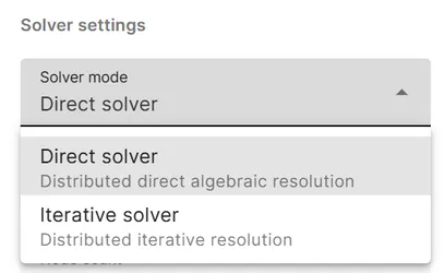
Solver settings

Two solver modes are available:

• Direct solver
  • Uses a regular parallelization scheme to solve the linear system.
• Iterative solver
  • Uses DDM to split the mesh into parts, which are then solved in parallel.

Solver mode options in the simulation settings

Direct solver

The direct solver solves the linear system of equations directly using standard matrix decomposition techniques. It leverages regular parallelization schemes to distribute the computational load across multiple CPUs or nodes.

Strengths	Limitations
Generally more robust and reliable, especially for smaller to medium-sized problems	Can be computationally expensive and memory-intensive for large problems
Typically provides a precise solution without requiring many iterations	Scalability can be limited for extremely large models due to memory constraints

Iterative solver

The iterative solver utilizes a Domain Decomposition Method (DDM) to split the mesh into smaller subdomains, which are solved independently and in parallel. The iterative solver then coordinates the solution between adjacent subdomains and continues iterating until the relative residual tolerance is met. Relative residual tolerance corresponds to the DDM convergence and not the solution convergence.

Strengths	Limitations
DDM enables efficient parallelization — each subdomain can be processed on a separate CPU or node	Convergence can be slower than with the direct solver, especially for ill-conditioned problems
More memory-efficient for large problems, as it only stores smaller subdomain matrices	Requires careful selection of solver parameters for optimal performance
Often scales better for very large models due to the distributed nature of DDM

Relative residual tolerance

The default Relative residual tolerance 1e-6 might be unnecessarily strict, leading to longer simulation runtimes.

For faster convergence, feel free to experiment with a lower tolerance, such as 1e-3. Keep in mind however, that this will lead to less accurate results.

Which one to choose?

The choice between direct and iterative solvers depends on the specific simulation:

• Smaller to medium-sized problems: The direct solver is often a good starting point due to its robustness and relative ease of use.
• Large-scale problems: The iterative solver with DDM can be more advantageous due to its memory efficiency and scalability.
• Complex geometries or highly coupled physics: For well-conditioned problems, the iterative solver is better suited to solve complex systems. The iterative solver is not suitable for ill-conditioned problems, however.
• Time constraints: If a quick solution is needed, a direct solver might be faster, especially if the problem size is manageable.

If you’re unsure, Allsolve has default settings that can provide a reasonable starting point. You can then experiment and compare the performance of both solvers to find the best fit for your specific simulation needs.