Elastic waves

This page describes the available interactions and couplings for elastic wave propagation in Allsolve. Use Elastic waves for harmonic or transient wave problems — ultrasound transducers, acoustic-structure coupling, and time-domain impulse response. For static deformation, contact, or large-deformation analysis, use Solid mechanics instead.

Weak formulation

The weak form solved by Allsolve is

\int_{\Omega}\; -\rho \boldsymbol{\ddot{u}} \cdot \boldsymbol{u}^\prime \; d\Omega + \int_{\Omega}\; -\boldsymbol{\sigma} \colon \boldsymbol{\varepsilon}^\prime \; d\Omega + \int_{\Omega}\; \boldsymbol{f} \cdot \boldsymbol{u}^\prime \; d\Omega + \int_{\Gamma}\; \boldsymbol{t} \cdot \boldsymbol{u}^\prime \; d\Gamma = 0.

where $\boldsymbol{u}$ is the displacement field, $\boldsymbol{\sigma}$ the stress tensor, $\boldsymbol{\varepsilon}$ the strain tensor, $\boldsymbol{t} = \boldsymbol{\sigma} \cdot \boldsymbol{n}$ the traction vector, $\boldsymbol{f}$ the body force, and $\rho$ the mass density. The inertia term $\rho \boldsymbol{\ddot{u}}$ makes this formulation suitable for time-dependent wave analysis.

See Formulation derivation for the full strong-to-weak derivation.

Elastic waves vs solid mechanics

Both physics use the displacement field $\boldsymbol{u}$ , but they target different analysis types.

Topic	Elastic waves	Solid mechanics
Primary use	Dynamic wave propagation (harmonic / transient)	Static, quasi-static, large-deformation
Analysis types	Harmonic, Transient, Eigenmode — not Static or Multiharmonic	Static, Harmonic, Multiharmonic, Transient, Eigenmode
Strain model	Linear small-strain only	Linear or Green–Lagrange (with geometric nonlinearity)
Wave-specific interactions	Absorbing boundary, PML, Continuity, Viscous damping, Viscoelastic material model	—
Structural-only interactions	—	Prestress, Geometric nonlinearity, Contact
Structural-only couplings	—	Magnetic force, Large displacement (mesh deformation)
Shared interactions	Load, Constraint, Clamp, Lump U/F, Pressure, Periodicity, Symmetry, Proportional damping	(same)
Shared couplings	Piezoelectricity, Thermal expansion, Electric force	(same)

Choose Elastic waves when you need to capture wave propagation, frequency response, or transient impulse behaviour. Choose Solid mechanics when deformation, stress, contact, or geometric nonlinearity is the primary concern.

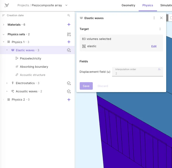
Setting up Elastic waves

Add Elastic waves to a physics set and assign a target region — the volumes where the wave equation is solved. The primary field is the displacement field ( $\boldsymbol{u}$ ). Set the interpolation order to control the polynomial degree of the finite-element basis (order 2 is typical for wave problems).

Elastic waves physics settings

Interactions

Load

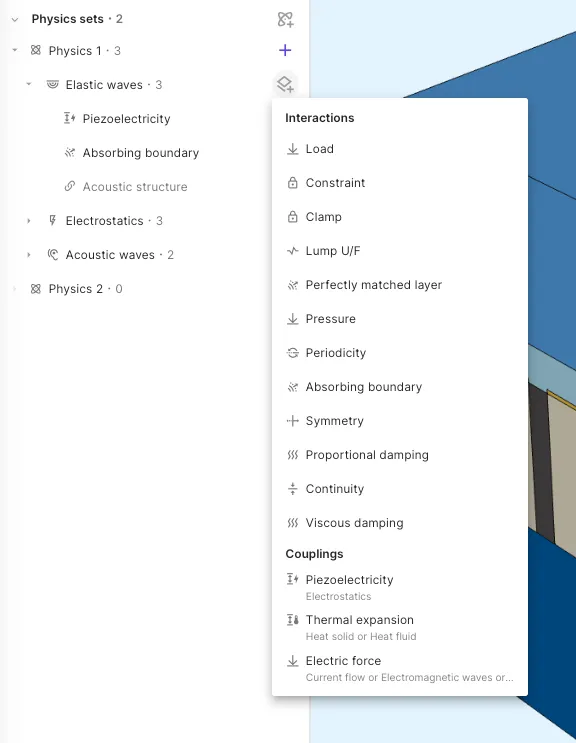
Applies an external mechanical load to a selected region by prescribing a force vector $\boldsymbol{f}$ , exciting the elastic domain and generating propagating waves.

Constraint

Fixes displacement components of the displacement field $\boldsymbol{u}$ . Use this interaction to fix displacements at a node, boundary, or within a region. Use Clamp to fix displacement values to zero.


How to use	You can use either the matrix editor or the expression editor. Matrix editor is the default — enable a dimension to constrain and enter the displacement value. With the expression editor, provide a `3×2` matrix with the first column containing `1` or `0` (whether a constraint is applied in that dimension or not), and the second column containing the displacement values.
Example	expression editor: `[0, 0; 1, 42; 0, 0]` applies a 3D displacement constraint of $u_y = 42$ in the y-direction, while the other dimensions remain unconstrained.
Unit	Displacement values in meters (m)

Clamp

Clamp is a special case of a Constraint where the displacement is fixed to zero. This boundary condition constrains all components of the displacement vector $\boldsymbol{u}$ in the targeted region to zero: $u_x = 0, u_y = 0, u_z = 0$

Lump U/F

Applies a lumped displacement $\boldsymbol{U}$ or force $\boldsymbol{F}$ through a boundary loop, replacing detailed field distribution with an equivalent lumped value. Commonly used to drive transducers with a prescribed voltage-derived displacement or a point force excitation.


How to use	Specify the target curve (must be a connected loop). From `Actuation mode`, select either displacement, force or circuit coupling. Use the matrix editor or the expression editor to define values: provide a `3×2` matrix for a 3D problem (`2×2` for 2D, etc.), where the first column contains `1` or `0` (whether a constraint is applied or not) and the second column contains the values.
Example	`[0, 0; 1, 0.01; 0, 0]` applies a 3D lumped displacement of $u_y = 0.01$ in the y-direction, while the other dimensions remain unconstrained.
Unit	Displacement values in meters (m) or force in Newtons (N)

Pressure

Applies a scalar pressure load normal to a boundary surface. Positive pressure acts inward (compression), negative pressure acts outward (tension). Unlike a general Load which requires specifying a force vector, Pressure only needs a scalar value — the direction is determined automatically from the surface normal.


How to use	Select the target boundary (surface for 3D, curve for 2D). Provide a scalar pressure value. Positive values push into the solid, negative values pull outward.
Example	`1e6` applies 1 MPa of compressive pressure to the selected surface.
Unit	Pressure in Pascals (Pa)

Periodicity

Imposes periodic boundary conditions for the displacement field $\boldsymbol{u}$ . Reduces computational domain size for problems with translational symmetry, such as unit-cell models of periodic arrays.


Example	Periodicity follows the same principles, regardless of which physics module it belongs to. See how periodicity is used in magnetism as a reference: Periodicity in electric motors

Symmetry

Imposes a symmetry boundary condition on a plane, constraining the normal displacement component to zero ( $u_n = 0$ ) while leaving tangential displacements free. Use this to model only a fraction of a symmetric structure (where both geometry and loads are symmetric about the cut plane), reducing computational cost.


How to use	Select the boundary that represents the symmetry plane.
Example	Cutting a beam with a centered load along its midplane and applying Symmetry to the cut face halves the number of degrees of freedom while producing the same result as the full model.

Proportional damping

Applies Rayleigh damping to the structure, where the damping matrix is a linear combination of the mass and stiffness matrices: $\boldsymbol{C} = \alpha \boldsymbol{M} + \beta \boldsymbol{K}$ . The mass-proportional coefficient $\alpha$ damps low-frequency modes, while the stiffness-proportional coefficient $\beta$ damps high-frequency modes.


How to use	Provide the mass damping coefficient $\alpha$ and the stiffness damping coefficient $\beta$ . These can be determined from known damping ratios at two reference frequencies.
Example	$\alpha = 0.1$ and $\beta = 0.001$ applies Rayleigh damping tuned to a target damping ratio across the frequency range of interest.
Unit	$\alpha$ in 1/s, $\beta$ in s

Perfectly matched layer

Implements an absorbing boundary region to simulate an infinite elastic domain and prevent reflections from truncated boundaries. Place PML at the outer boundary of the elastic domain where outgoing waves should exit without reflection.

Two types are available:

AML type — suitable for smooth or curved boundaries.
Box PML — suitable for rectangular or cornered boundaries.

The number of PML layers can be tuned in the Shared PML settings.

Absorbing boundary

Applies a first-order absorbing boundary condition to truncate the computational domain, allowing outgoing elastic waves to pass through with minimal reflection. Lighter-weight than a Perfectly matched layer — suitable when a simpler setup is acceptable and some small residual reflection is tolerable.


How to use	Select the outer boundary of the elastic domain where waves should exit. No additional parameters are needed — the condition automatically matches the mechanical impedance of the medium.

Continuity

Ensures continuity of the displacement field $\boldsymbol{u}$ across an interface between two boundaries. Used to map the elastic field continuously across mismatched or sliding mesh interfaces.


Example	Continuity follows the same principles, regardless of which physics module it belongs to. See how continuity is used in magnetism as a reference: Continuity in electric motors

Viscous damping

Applies viscous damping within a region, modelling energy dissipation as elastic waves propagate. Use this to represent material damping or attenuation in the bulk domain.


How to use	Select the target region and set the damping coefficient.

Viscoelastic material model

Enables viscoelastic behaviour in a region by activating the Prony series defined on the material. Use this for time-dependent relaxation and creep in polymers, adhesives, or other viscoelastic solids.


How to use	Select the target region where the viscoelastic material is assigned. Define the Prony series on the material (relaxation times and moduli).
Example	MEMS 003 — Viscoelasticity benchmark

Couplings to Other Physics

Elastic waves supports the following couplings:

Piezoelectricity
- Couples to Electrostatics
- Select target region of piezoelectric material such as PZT as target
Thermal expansion
- Heat solid
- Heat fluid
Electric force
- Current flow
- Electromagnetic waves
- Electrostatics
- Magnetism H

To couple an elastic solid to a fluid acoustic domain, add the Acoustic structure coupling from the Acoustic waves physics.

Compatibilities with analysis types

Elastic waves supports Harmonic, Transient, and Eigenmode analysis. Static analysis is not applicable. Multiharmonic analysis is not supported.

See the full compatibility table in Simulations overview.

Use cases

Elastic waves — PMUT array (piezoelectricity + acoustic structure)
Elastic waves — Piezocomposite transducer (transient wavelet excitation)
Elastic waves — Viscoelasticity benchmark (viscoelastic material model)

Formulation derivation

Elastic waves uses the same Cauchy momentum equation as solid mechanics, but always with the linear small-displacement strain tensor and the inertia term retained for time-dependent analysis.

Strong formulation

The strong form of deformable solids is given by the Cauchy momentum equation

\begin{align*} \nabla \cdot \boldsymbol{\sigma} + \boldsymbol{f} = \rho \boldsymbol{\ddot{u}} \tag{1} \end{align*}

where

$\boldsymbol{\sigma}$ is the stress tensor
$\boldsymbol{f}$ is the volumetric body force vector
$\rho$ is the mass density
$\boldsymbol{u}$ is the displacement field vector
$\boldsymbol{\ddot{u}}$ is the acceleration vector

Constitutive equation

Generalized Hooke’s law defines the relation between the stress and strain components

\boldsymbol{\sigma} = \boldsymbol{C} \boldsymbol{\varepsilon},

where $\boldsymbol{C}$ is a fourth-order elasticity tensor and $\boldsymbol{\varepsilon}$ is the strain tensor.

Strain tensor

Elastic waves uses the linear small-displacement strain tensor:

\boldsymbol{\varepsilon} = \dfrac{1}{2} \left( \nabla \boldsymbol{u} + (\nabla \boldsymbol{u})^T \right)

Voigt notation

In Voigt notation, the stress and strain tensors are represented as vectors. Consequently, the constitutive relation takes the form

\boldsymbol{\sigma}_v = \boldsymbol{H} \boldsymbol{\varepsilon}_v,

where $\boldsymbol{H}$ is the elasticity matrix which is a symmetric $6 \times 6$ matrix.

Deriving the weak form

To obtain the weak form, multiply $\text{(1)}$ by the test function $\boldsymbol{u}^\prime$ and integrate over the domain $\Omega$ :

\int_{\Omega}\; -\rho \boldsymbol{\ddot{u}} \cdot \boldsymbol{u}^\prime \; d\Omega + \int_{\Omega}\; (\nabla \cdot \boldsymbol{\sigma}) \cdot \boldsymbol{u}^\prime \; d\Omega + \int_{\Omega}\; \boldsymbol{f} \cdot \boldsymbol{u}^\prime \; d\Omega = 0

Applying Leibniz rule on the divergence term, we get

\int_{\Omega}\; -\rho \boldsymbol{\ddot{u}} \cdot \boldsymbol{u}^\prime \; d\Omega + \int_{\Omega}\; -\boldsymbol{\sigma} \colon \nabla \boldsymbol{u}^\prime \; d\Omega + \int_{\Omega}\; \nabla \cdot (\boldsymbol{\sigma} \cdot \boldsymbol{u}^\prime) \; d\Omega + \int_{\Omega}\; \boldsymbol{f} \cdot \boldsymbol{u}^\prime \; d\Omega = 0.

Applying Divergence theorem on the divergence term, we get

\int_{\Omega}\; -\rho \boldsymbol{\ddot{u}} \cdot \boldsymbol{u}^\prime \; d\Omega + \int_{\Omega}\; -\boldsymbol{\sigma} \colon \nabla \boldsymbol{u}^\prime \; d\Omega + \int_{\Gamma}\; \boldsymbol{u}^\prime \cdot (\boldsymbol{\sigma} \cdot \boldsymbol{n}) \; d\Gamma + \int_{\Omega}\; \boldsymbol{f} \cdot \boldsymbol{u}^\prime \; d\Omega = 0.

Since the stress tensor is symmetric, the following relation holds.

\begin{align*} \boldsymbol{\sigma} \colon \nabla \boldsymbol{u}^\prime &= \boldsymbol{\sigma} \colon (\nabla {\boldsymbol{u}^\prime})^T \\ &= \boldsymbol{\sigma} \colon \dfrac{1}{2} \left((\nabla {\boldsymbol{u}^\prime})^T + (\nabla {\boldsymbol{u}^\prime})^T \right) \\ &= \boldsymbol{\sigma} \colon \dfrac{1}{2} \left(\nabla {\boldsymbol{u}^\prime} + (\nabla {\boldsymbol{u}^\prime})^T \right) \\ &= \boldsymbol{\sigma} \colon \boldsymbol{\varepsilon}^\prime \end{align*}

Substituting $\boldsymbol{\sigma} \colon \nabla \boldsymbol{u}^\prime = \boldsymbol{\sigma} \colon \boldsymbol{\varepsilon}^\prime$ and following the definition of traction vector $\boldsymbol{t} = \boldsymbol{\sigma \cdot n}$ , we get the final weak formulation stated at the top of this page.