
PMSM 2D torque analysis - EM 001
Prerequisites: complete the PMSM electric motor tutorial first — it covers the 3D version of this motor and introduces remanence, periodicity, and torque calculation in detail.
In this demo, we simulate a 2D cross-section of a Permanent Magnet Synchronous Motor (PMSM) to analyze how torque varies with the mechanical angle. The goal is to demonstrate how to set up the simulation efficiently using Allsolve.
PMSMs are widely used in electric vehicles and automation due to their high efficiency and precise control. Simulating their behavior helps:
- Optimize torque ripple and smoothness
- Accelerate motor design through virtual prototyping
An additional goal of this demo is to illustrate the modifications required to support 2D simulations.
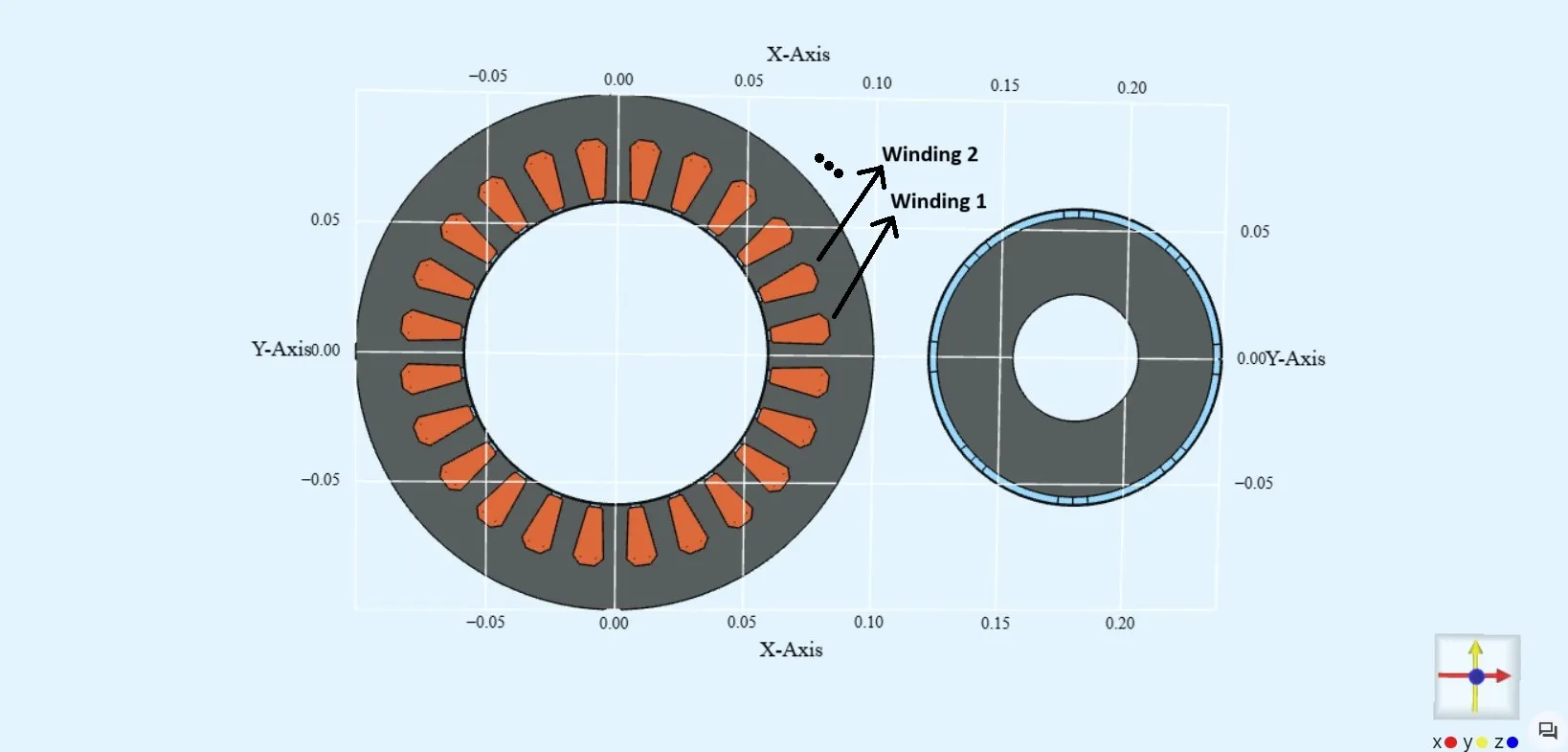
Model definitions
Section titled “Model definitions”Stator
Section titled “Stator”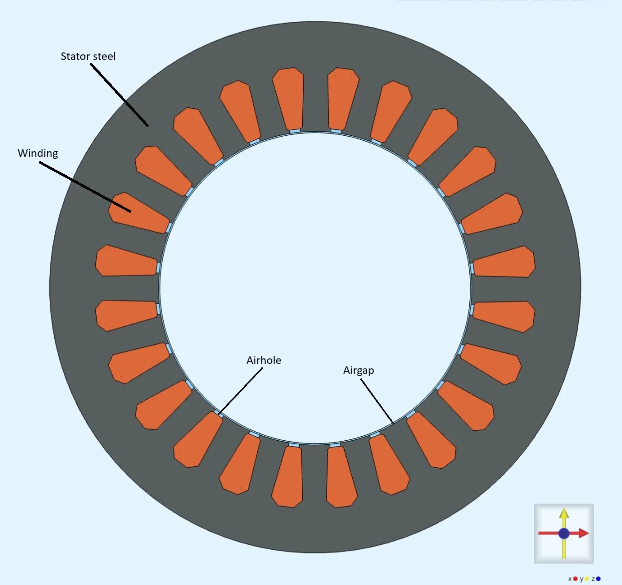
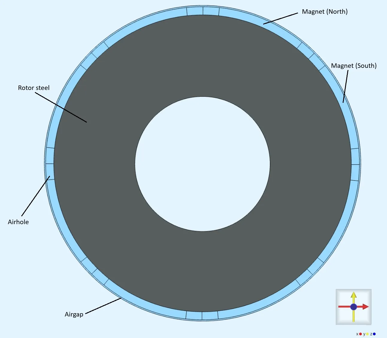
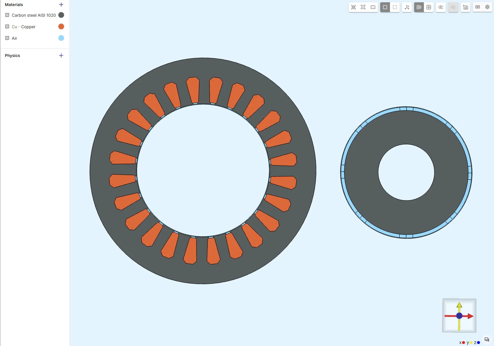
Step 1 – Build the Geometry
Section titled “Step 1 – Build the Geometry”- Import a .STEP file of the PMSM 2D cross-section. File download link: pmsm-2D-electric-motor.step
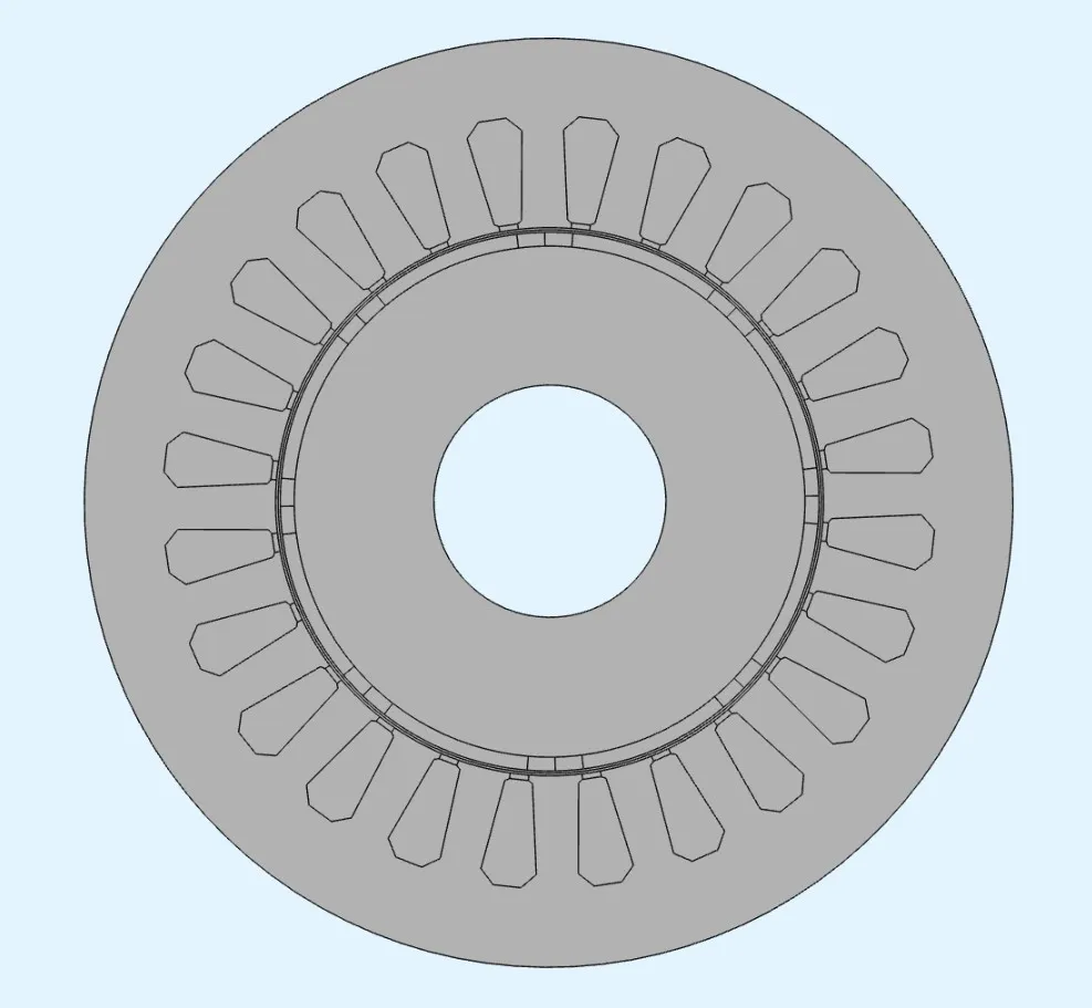
- Use Translate to move the rotor outward (e.g.,
0.18 malong x-axis) to prepare for separate meshing.
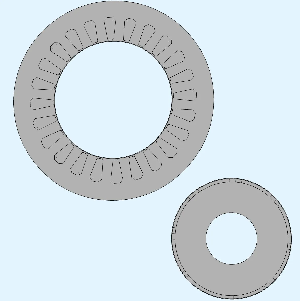
Lock the geometry and proceed to Physics.
Step 2 – Apply Physics
Section titled “Step 2 – Apply Physics”Define Surface Regions
Section titled “Define Surface Regions”Go to: Common → Definitions → Region → Surface
and define the following surface regions to simplify later steps:
| Region Name | Notes |
|---|---|
rotor |
All rotor parts |
airgap |
Each one from rotor and stator side, don’t include airholes |
magnet_s |
All south pole magnets |
magnet_n |
All north pole magnets |
magnetism_H |
All windings |
magnetism_phi |
All but windings |
Assign Materials
Section titled “Assign Materials”| Part | Material | Notes |
|---|---|---|
| Rotor & Stator | Carbon Steel AISI 1020 | Use linear μ: 2000 * mu0 |
Windings (magnetism_H) |
Copper | |
| Remaining domains | Air |
Define Simulation Variables
Section titled “Define Simulation Variables”Go to Common → Definitions → Variables and add New variables:
| Name | Description | Expression |
|---|---|---|
I |
Current amplitude (A) | 300 |
alpha |
Mechanical angle (°) | 0 |
theta |
Electrical angle (°) | 0 |
Step 3 - Add Magnetism φ interactions
Section titled “Step 3 - Add Magnetism φ interactions”- Apply
Magnetism φto all parts except copper windings.
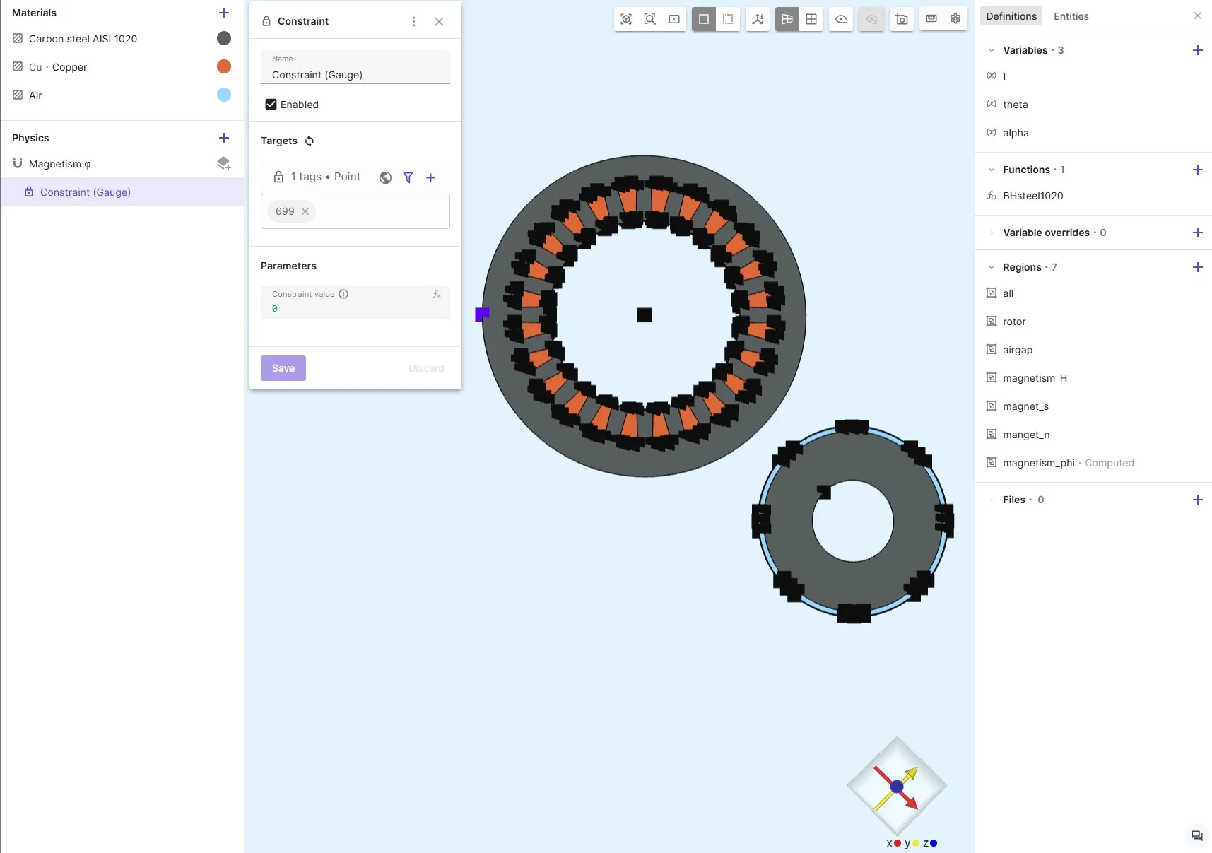
Gauge Constraint
Section titled “Gauge Constraint”- Add a constraint to ensure a unique solution.
- Set value =
0at a point on the outer edge.
Airgap Continuity
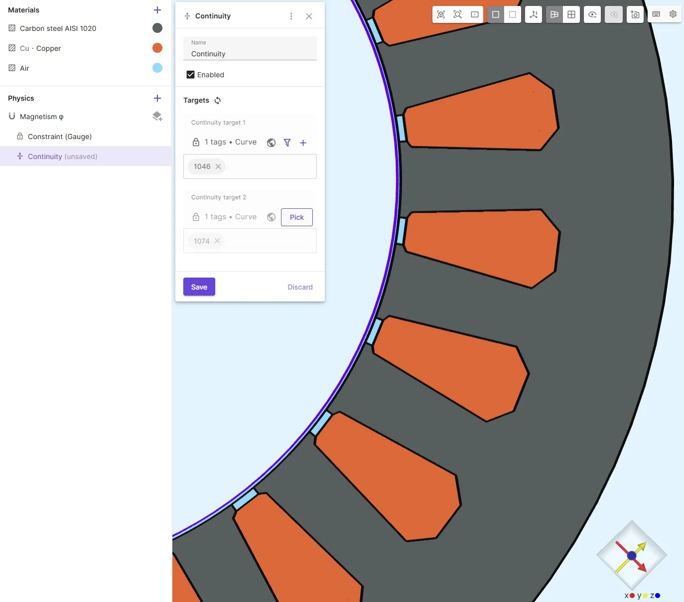
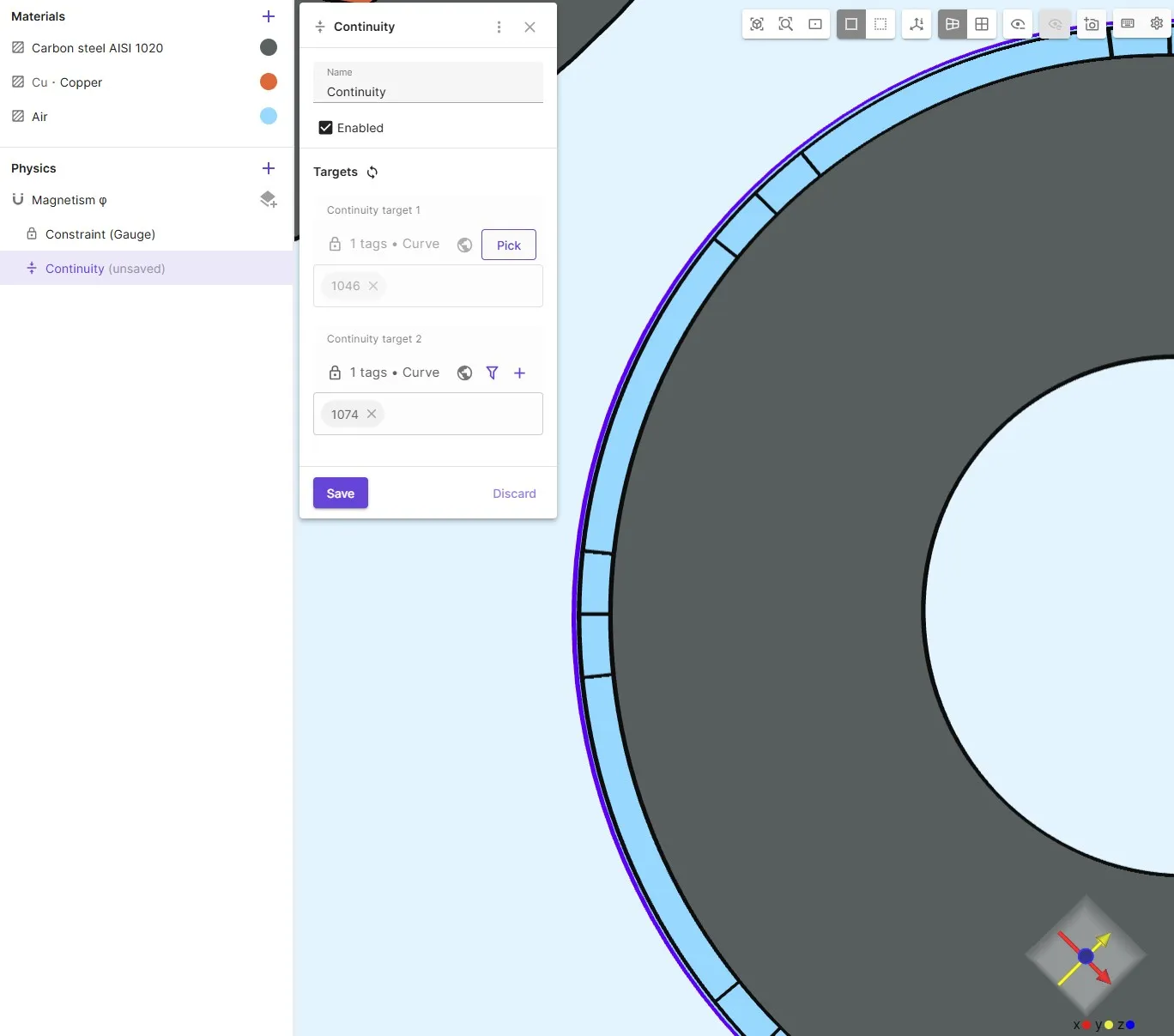
Section titled “Airgap Continuity”- Add
Continuitycondition across rotor-stator interface. - Target 1 = stator side curve
Target 2 = rotor side curve
Order matters !
Stator
Rotor
Apply Stator Currents
Section titled “Apply Stator Currents”To generate a rotating magnetic field, apply phase currents with Lump I/V cut to windings:
- Number windings 1–24 counter-clockwise starting at +x direction.
- Assign regions:
wind1,wind2, …,wind24 - Assign namespaces:
lump1,lump2, …,lump24
For now, set current = 0 — we’ll define values later via scripting.
Add Remanence (Permanent magnets)
Section titled “Add Remanence (Permanent magnets)”-
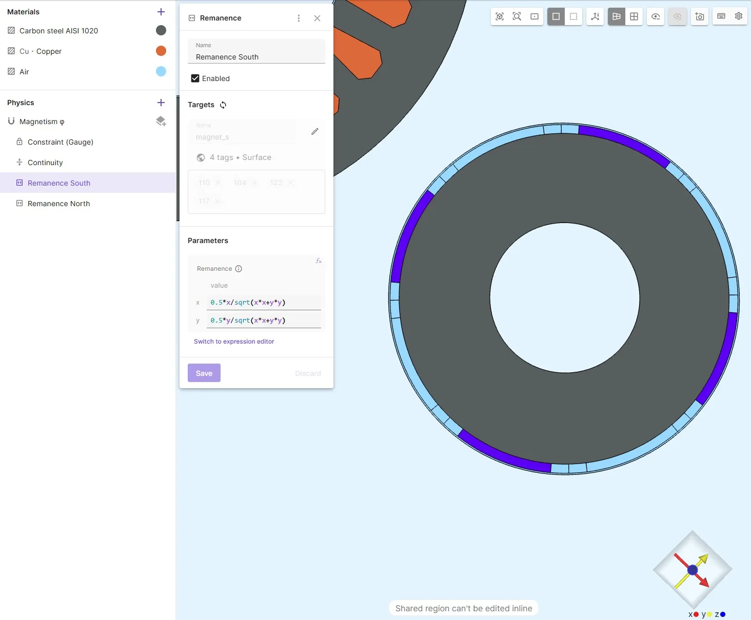
Add radial magnetization to the permanent magnets using given formulas.
Note: Ensure that the South pole is facing windings 1, 2, and 3 to create an attractive force between the permanent magnets and the windings. Otherwise the motor is not rotating correctly.
| Region | Remanence Vector Expression |
|---|---|
magnet_s |
[0.5*x/sqrt(x^2+y^2); 0.5*y/sqrt(x^2+y^2)] |
magnet_n |
[-0.5*x/sqrt(x^2+y^2); -0.5*y/sqrt(x^2+y^2)] |
Step 4 - Add Magnetism H interactions
Section titled “Step 4 - Add Magnetism H interactions”Couple the interactions
Section titled “Couple the interactions”- Apply
Magnetism Hto all windings - Couple the
Magnetism Hwith theMagnetism φ
Step 5 – Mesh Settings
Section titled “Step 5 – Mesh Settings”Mesh Settings
Section titled “Mesh Settings”- Enable Curved mesh.
- Open the collapsible menu for
Mesh element size. - Set Max size to
0.005. - Under
Customizations, add a Mesh refinement for airgap:- Set Max size to
0.0001.
- Set Max size to
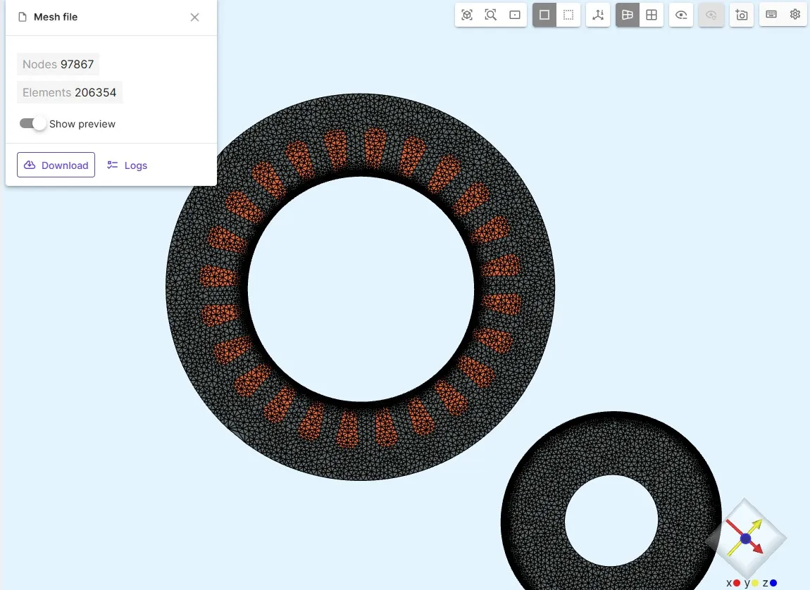
Refining the airgap is crucial for accurate torque integration.
Step 6 – Simulation Setup
Section titled “Step 6 – Simulation Setup”- Use Steady-State solver
- Add physics:
Magnetism φandMagnetism H - Add generated mesh
- Keep other settings at default
Step 7 – Modifying Autogenerated Script
Section titled “Step 7 – Modifying Autogenerated Script”To simulate rotor movement dynamically, first reverse the initial static translation, then apply rotation by mechanical angle alpha.
Insert the following lines right after the mesh.mesh.load() call:
# Reverse static shifttranslation_x = 0.18mesh.mesh.shift(reg.rotor, -translation_x, 0.0, 0.0)# Apply dynamic rotationmesh.mesh.rotate(reg.rotor, 0.0, 0.0, expr.alpha)Adapt Field Vectors for 3D Calculations
Section titled “Adapt Field Vectors for 3D Calculations”Although this is a 2D simulation, the solver’s algorithms use 3D vectors. Therefore, we must update some of the default 2x1 vectors to 3x1 vectors by adding a zero to the z-dimension.
First, modify the parameter definitions for the magnetic field components:
df.H = qs.parameter(3, 1) # Magnetic field vector (Hx, Hy, Hz=0)df.B = qs.parameter(3, 1) # Magnetic flux density vectordf.j = qs.parameter(3, 1) # Current density vectordf.E = qs.parameter(3, 1) # Electric field vectorNext, update the Magnetic field and Magnetic flux density definitions. This involves resizing the gradient of the magnetic scalar potential (fld.phi) and converting the remanence flux density arrays from qs.array2x1 to qs.array3x1.
Magnetic field
Section titled “Magnetic field”df.H.addvalue(qs.selectunion([reg.magnetism_h, reg.magnetism_phi]), -qs.grad(fld.phi).resize(3,1))df.H.addvalue(reg.magnetism_h, fld.H)df.H.addvalue(qs.selectunion([reg.magnetism_h, reg.magnetism_phi]), var.Hs)Magnetic flux density
Section titled “Magnetic flux density”df.B.addvalue(qs.selectunion([reg.magnetism_h, reg.magnetism_phi]), -par.mu() * qs.grad(fld.phi).resize(3,1))df.B.addvalue(reg.magnetism_h, par.mu() * fld.H)df.B.addvalue(qs.selectunion([reg.magnetism_h, reg.magnetism_phi]), par.mu() * var.Hs)df.B.addvalue(reg.magnet_n, qs.array3x1(-0.5 * qs.getx() / qs.sqrt(qs.getx() * qs.getx() + qs.gety() * qs.gety()), -0.5 * qs.gety() / qs.sqrt(qs.getx() * qs.getx() + qs.gety() * qs.gety()), 0))df.B.addvalue(reg.magnet_s, qs.array3x1(0.5 * qs.getx() / qs.sqrt(qs.getx() * qs.getx() + qs.gety() * qs.gety()), 0.5 * qs.gety() / qs.sqrt(qs.getx() * qs.getx() + qs.gety() * qs.gety()), 0))Define Winding Currents
Section titled “Define Winding Currents”To generate a rotating magnetic field, you must define the sinusoidal currents for each phase of the motor windings. The following code block sets up three-phase currents (A, B, C) with a 60-degree phase shift.
Replace the entire auto-generated Lump I/V cut interactions section with the code below. This assumes the windings were created and named with identical namespaces.
# Define current phasesA = 0B = 60C = 120
# Lump I/V cut interactions for all 24 windingsform += port.lump1.I - expr.I * qs.sin((expr.theta + 4.0 * expr.alpha - A) * qs.getpi() / 180.0)form += port.lump2.I - expr.I * qs.sin((expr.theta + 4.0 * expr.alpha - B) * qs.getpi() / 180.0)form += port.lump3.I - expr.I * qs.sin((expr.theta + 4.0 * expr.alpha - C) * qs.getpi() / 180.0)form += port.lump4.I + expr.I * qs.sin((expr.theta + 4.0 * expr.alpha - A) * qs.getpi() / 180.0)form += port.lump5.I + expr.I * qs.sin((expr.theta + 4.0 * expr.alpha - B) * qs.getpi() / 180.0)form += port.lump6.I + expr.I * qs.sin((expr.theta + 4.0 * expr.alpha - C) * qs.getpi() / 180.0)form += port.lump7.I - expr.I * qs.sin((expr.theta + 4.0 * expr.alpha - A) * qs.getpi() / 180.0)form += port.lump8.I - expr.I * qs.sin((expr.theta + 4.0 * expr.alpha - B) * qs.getpi() / 180.0)form += port.lump9.I - expr.I * qs.sin((expr.theta + 4.0 * expr.alpha - C) * qs.getpi() / 180.0)form += port.lump10.I + expr.I * qs.sin((expr.theta + 4.0 * expr.alpha - A) * qs.getpi() / 180.0)form += port.lump11.I + expr.I * qs.sin((expr.theta + 4.0 * expr.alpha - B) * qs.getpi() / 180.0)form += port.lump12.I + expr.I * qs.sin((expr.theta + 4.0 * expr.alpha - C) * qs.getpi() / 180.0)form += port.lump13.I - expr.I * qs.sin((expr.theta + 4.0 * expr.alpha - A) * qs.getpi() / 180.0)form += port.lump14.I - expr.I * qs.sin((expr.theta + 4.0 * expr.alpha - B) * qs.getpi() / 180.0)form += port.lump15.I - expr.I * qs.sin((expr.theta + 4.0 * expr.alpha - C) * qs.getpi() / 180.0)form += port.lump16.I + expr.I * qs.sin((expr.theta + 4.0 * expr.alpha - A) * qs.getpi() / 180.0)form += port.lump17.I + expr.I * qs.sin((expr.theta + 4.0 * expr.alpha - B) * qs.getpi() / 180.0)form += port.lump18.I + expr.I * qs.sin((expr.theta + 4.0 * expr.alpha - C) * qs.getpi() / 180.0)form += port.lump19.I - expr.I * qs.sin((expr.theta + 4.0 * expr.alpha - A) * qs.getpi() / 180.0)form += port.lump20.I - expr.I * qs.sin((expr.theta + 4.0 * expr.alpha - B) * qs.getpi() / 180.0)form += port.lump21.I - expr.I * qs.sin((expr.theta + 4.0 * expr.alpha - C) * qs.getpi() / 180.0)form += port.lump22.I + expr.I * qs.sin((expr.theta + 4.0 * expr.alpha - A) * qs.getpi() / 180.0)form += port.lump23.I + expr.I * qs.sin((expr.theta + 4.0 * expr.alpha - B) * qs.getpi() / 180.0)form += port.lump24.I + expr.I * qs.sin((expr.theta + 4.0 * expr.alpha - C) * qs.getpi() / 180.0)
Finally, resize the remaining gradient terms in the Magnetism φ and H-φ coupling interaction sections to ensure full 3D vector compatibility.
Magnetism φ
# Magnetism φform += qs.integral(reg.magnetism_phi, -par.mu() * (qs.grad(qs.dof(fld.phi)).resize(3,1) - var.dof_Hs) * qs.grad(qs.tf(fld.phi)).resize(3,1))H-φ coupling
# H-φ coupling interactionvar.phi_dofs_reg = qs.selectunion([reg.magnetism_phi, reg.magnetism_h])form += qs.integral(reg.magnetism_h, -par.mu() * qs.grad(qs.dt(qs.dof(fld.phi, var.phi_dofs_reg))).resize(3,1) * qs.tf(fld.H))form += qs.integral(reg.magnetism_h, -par.mu() * (qs.dt(qs.dof(fld.H)) + var.dt_dof_Hs - qs.grad(qs.dt(qs.dof(fld.phi, var.phi_dofs_reg))).resize(3,1)) * var.tf_Hs)form += qs.integral(reg.magnetism_phi, -par.mu() * (var.dt_dof_Hs - qs.dt(qs.grad(qs.dof(fld.phi))).resize(3,1)) * var.tf_Hs)form += qs.integral(reg.magnetism_h, par.mu() * (qs.dof(fld.H) - qs.grad(qs.dof(fld.phi, var.phi_dofs_reg)).resize(3,1) + var.dof_Hs) * qs.grad(qs.tf(fld.phi, var.phi_dofs_reg)).resize(3,1))Calculate Torque and Define Outputs
Section titled “Calculate Torque and Define Outputs”Add the following post-processing code after the form.allsolve() command to compute the torque. Two common methods, Arkkio’s method and the Maxwell stress tensor, are included for result verification.
# Arkkio's methodrs = 0.059 # outer radius of airgap [m]rr = 0.058 # inner radius of airgap [m]z_length = 0.05 # thickness of motor slice [m]radius = qs.sqrt( qs.pow(qs.getx(),2) + qs.pow(qs.gety(),2) )ephi = qs.array3x1(-qs.gety()/radius, qs.getx()/radius, 0)er = qs.array3x1(qs.getx()/radius, qs.gety()/radius, 0)Bphi = df.B*ephiBr = df.B*erdr = (rs-rr)magforcedensity1 = (z_length*radius*Br*Bphi/qs.getmu0()/dr)torque1 = magforcedensity1.allintegrate(reg.airgap, 2)
# Maxwell stress tensor methodleverarm = qs.array3x1(qs.getx(), qs.gety(), 0.0)T = 1/qs.getmu0() * ( df.B*qs.transpose(df.B) - 0.5*df.B*df.B * qs.eye(3))magforcedensity2 = qs.on(reg.airgap, T)*qs.normal(reg.airgap).resize(3,1)torque2 = -z_length*qs.compz(qs.crossproduct(leverarm, magforcedensity2)).allintegrate(reg.continuity_target_1, 2)
To visualize simulation results and assist with debugging, add the following output definitions at the very end of your script.
qs.setoutputvalue("Angle", qs.evaluate(qs.evaluate(expr.alpha)[0]))qs.setoutputvalue("Torque (Arkkio)", qs.evaluate(torque1))qs.setoutputvalue("Torque (Maxwell's Stress Tensor)", qs.evaluate(torque2))
# Field outputsqs.setoutputfield("B", reg.all, df.B, 2)qs.setoutputfield("j", reg.magnetism_h, df.j, 1)
# Winding current outputsqs.setoutputvalue("I_phase1", qs.evaluate(port.lump1.I))qs.setoutputvalue("I_phase2", qs.evaluate(port.lump2.I))qs.setoutputvalue("I_phase3", qs.evaluate(port.lump3.I))
Step 8 – Run the Simulation Sweep
Section titled “Step 8 – Run the Simulation Sweep”To analyze the motor’s performance over different rotor positions, run the simulation across a range of mechanical angles.
- Navigate to
Common → Definitions → Variable Overrides → Sweep. - Add a sweep for the mechanical angle variable
alpha. - A typical sweep range is from 0 to 45 degrees (e.g., [0, 1, 2, …, 45]) since the torque cycle repeats every 45 degrees.
Step 9 - Run and Plot Results:
Section titled “Step 9 - Run and Plot Results:”Torque
Section titled “Torque”- Include the sweep you created as an input to the simulation.
- Run the simulation over the specified range.
- Once complete, go to the
Plotsection. - Create a graph plotting the calculated torque as a function of mechanical angle.
The resulting plot should resemble this:
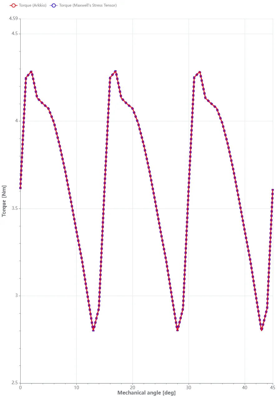
You should observe the torque curves from both calculation methods overlaid, oscillating around a mean torque of approximately 3.5 Nm.
These results align well with the reference implementation documented in the Sparselizard documentation.
Magnetic Flux Density
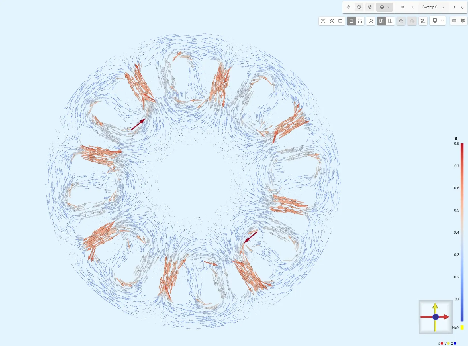
Section titled “Magnetic Flux Density”The magnetic flux density B in the core region can be visualized using a simple Glyph plot created via the Visualization module. The plot illustrates the direction and relative magnitude of the flux density, which reaches values under 1 T.
References
Section titled “References”Arkkio’s Method for Torque Computation, https://www.anttilehikoinen.fi/research-work/arkkios-method-torque-computation/
This simulation was created based on the provided Sparselizard example, https://github.com/halbux/sparselizard/blob/master/examples/electric-motor-pmsm-2d/main.cpp