Results

What you’ll learn

• Summary: Track value outputs across timesteps and sweep subsimulations.
• Plotting: Plot value outputs with configurable axes and series grouping.
• Visualizations: Visualize field output distributions over the simulation domain.

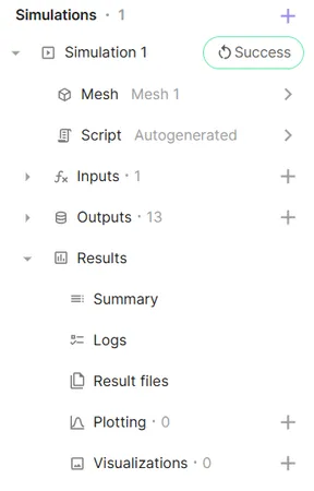
After a simulation starts running, Results become available.

The Results section contains 5 subsections:

• Summary
• Logs
• Result files
• Plotting
• Visualizations

Summary

The Summary lists all value outputs. Value outputs are shown for each transient simulation timestep or sweep subsimulation.

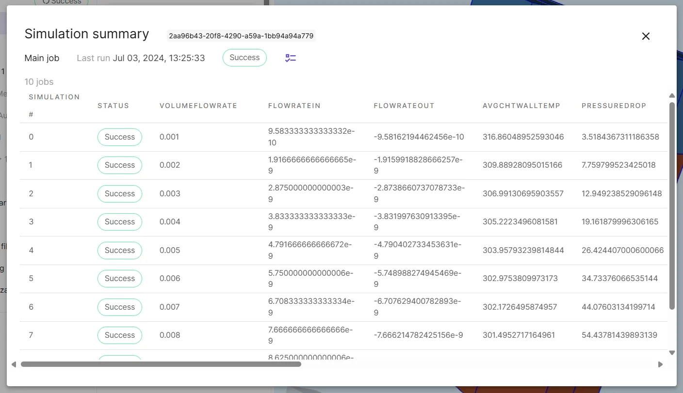
If an error occurs and a simulation run fails, you can check the summary status column to see at what point it occurred. Value outputs can also be exported as a .csv table from the summary.

Logs

Status messages sent during simulation runs appear in the Logs. The simulation log shows what happens during a simulation run.

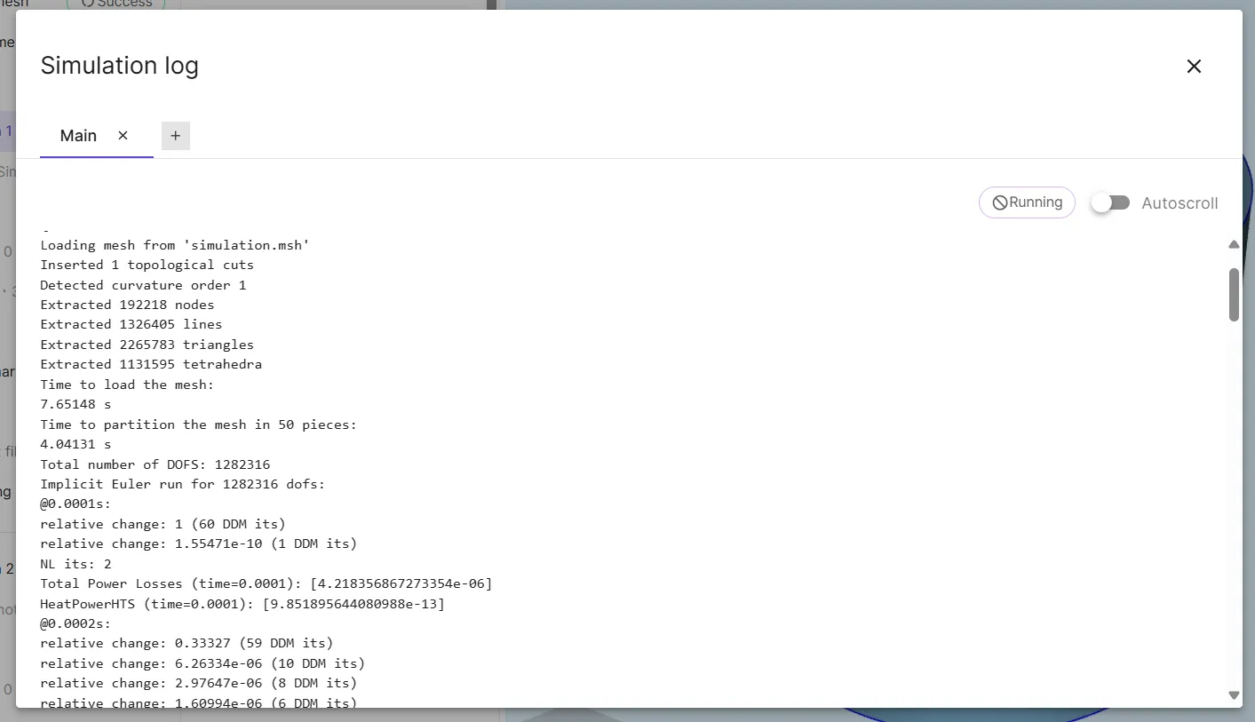
Values can also be printed to the Logs with the print function in script.

For a closer look at logs, see the dedicated page Simulation log.

Result files

Result files contains downloadable simulation results in .vtu or .json format.

Plotting

Plotting displays simulation value outputs as charts.

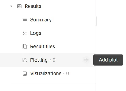
To add a plot, select + next to Plotting:

A new plot starts with one empty series. A single plot can have any number of series.

Series options include:

• Data source
  • Which simulation provides the data.
• X value
  • Value to plot on the X-axis.
• Y value
  • Value to plot on the Y-axis.
• Series from
  • Optional.
  • Available when data dimensions exceed 2, for example in transient sweep simulations.
  • Groups data by a dimension, such as sweep step, and creates series from the groups automatically.
• Bound input
  • Optional.
  • Available when data dimensions exceed 3, for example in transient sweeps when plotting array values.
  • Binds a data dimension, such as array index, to enable plotting multidimensional data.

Plot configuration

The plot settings can be further customized in the Customization tab. Some notable settings are described below.

To get crisp plots, set General > Plot rendering to SVG before saving an image of the plot.

Series type can be set individually for each series or shared for all series under Series > Series type. Supported types are line, bar, and scatter.

By default, undefined output data points break the line plot. Turn on Connect over nulls to connect between defined points.

Visualizations

Visualizations displays field outputs over the simulation domain. Field outputs are either added as simulation outputs or written in custom script with the setoutputfield function.

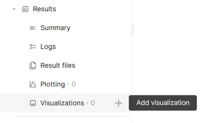
To add a visualization, select + next to Visualizations:

Select one or more source fields to visualize.

Tip

General model view controls (camera rotation, zoom, hide surfaces, measure, screenshot) are shared across all visualizer modes. See Model view controls for reference.

Adding a visualization

1. Select + next to Visualizations.
2. Choose a source field from the field picker. Multiple sources can be added to a single visualization.
3. Select Activate current visualization to connect to a visualizer server and load the processed data.

Filter stack

A visualization is structured as a pipeline. Source fields form the base; filters are applied on top in sequence. Each filter transforms the output of the item below it in the stack.

To add a filter, select Add filter on the visualization item. The new filter is inserted above the current selection.

Filter	Purpose
Warp	Displaces the mesh by a vector field, scaled by a factor
Warp by scalar	Displaces the mesh along a chosen direction by scalar field values
Slice	Cuts the domain with a plane, showing the field on the cross-section
Clip	Removes geometry on one side of a plane
Threshold	Shows only elements where field values fall within a specified range
Contour	Extracts iso-surfaces at specified field values
Streamline	Traces flow paths through a vector field
Glyph	Places arrow or line symbols representing vector direction and magnitude

Select Render in the toolbar to apply changes after modifying the filter stack or its parameters.

Filter settings

Each filter has configurable parameters accessible from its settings.

Source

Parameter	Description
Field	The source field (read-only).
Merge style	How multi-rank data is combined. Clean to grid merges overlapping partition data onto a regular grid, producing a smooth continuous field — best for most visualizations. Tessellate stitches partition meshes together with linearly interpolated field values that closely approximate the original field while splitting higher order tets to first order. None keeps each partition as a separate block with no merging, which can reveal partition boundaries and per-rank differences.
Component	For vector fields, select which component to visualize: Magnitude, X, Y, or Z.

Warp

Parameter	Description
Scale factor	Multiplier for the displacement. Use Reset to current data to auto-scale based on max field magnitude.

Warp requires a vector field as input. The mesh is displaced in the direction of the vector at each point, multiplied by the scale factor.

Warp by scalar

Parameter	Description
Scale factor	Multiplier for the displacement magnitude.
Direction	Direction of displacement: X, Y, Z, or Surface normal.

Slice

Parameter	Description
Origin	Position of the cutting plane center. Use Reset to data bounds to return to center.
Normal	Plane orientation. Preset buttons: X, Y, Z, Camera.
Show plane	Toggle visibility of the cutting plane widget in the viewport.
Cut by full cells	When enabled, preserves whole cells that the plane intersects rather than interpolating a smooth cut.

The cutting plane can also be repositioned interactively using the plane widget in the viewport.

Clip

Parameter	Description
Origin	Position of the clipping plane center.
Normal	Plane orientation. Preset buttons: X, Y, Z, Camera.
Cut by full cells	Preserves whole cells at the boundary.
Invert	Reverses which side of the plane is kept.

Threshold

Parameter	Description
Threshold type	Absolute (raw field values), Relative to range (percentage of min–max), or Relative to Z-score (standard deviations from mean).
Show values	Which portion to display: Above, Below, or Between the thresholds.
Lower threshold	Lower bound value.
Upper threshold	Upper bound value.

Contour

Parameter	Description
Mode	Count — evenly spaced iso-surfaces, or Values — explicit iso-values.
Number of contours	How many iso-surfaces to extract (Count mode).
Values	Comma-separated field values at which to extract iso-surfaces (Values mode).

Streamline

Parameter	Description
Integration direction	forward, backward, or both.
Seed type	Geometry that defines starting points: line or pointCloud.
Resolution	Number of seed points along the line (line seed).
Line point 1 / Line point 2	Coordinates of the seed line endpoints.
Number of points	Total seed points (point cloud).
Center / Radius	Position and extent of the point cloud sphere.

Streamlines require a vector field as input.

Glyph

Parameter	Description
Glyph mode	Shape of the glyph: arrow or line.
Scaling mode	Scale by geometry (uniform size) or data (proportional to field magnitude).
Scale factor	Size multiplier. Use Reset to current data to auto-scale.
Max sample points	Limits the number of glyphs to avoid visual clutter and performance issues.

Glyphs require a vector field as input.

Coloring and layers

Each filter output exposes one colorable field called layer. A layer can be point data or cell data, scalar or vector.

Switching layers

When multiple layers are available, use the Previous layer / Next layer buttons in the result toolbar to cycle through them. The active layer name is displayed between the buttons.

Configuring a layer

Open the layer configuration from the filter settings panel:

Setting	Description
Layer	Select which field array to color by.
Color preset	Color map to apply. Available presets: Cool to Warm, 2hot, Rainbow Desaturated, Grayscale.
Log scale	Toggle between linear and logarithmic color mapping.
Min / Max	Clamp the color range. Use Reset to data min / Reset to data max to restore full-range mapping.

Vector component selection

For vector field layers, the Component setting on the source filter controls which component is visualized: Magnitude, X, Y, or Z.

Tools

Main result tools

1. Refresh visualization
2. Probe
3. Show model
4. Rendering style
5. Change layer displayed in the scalar bar

Probe

Select Probe result point data in the result toolbar to activate the probe tool. Hover over the model to read field values at the pointed location. The probed values appear in an overlay at the bottom of the viewport.

Select the probe button again to deactivate.

Show model

Select Show model to overlay the input geometry along with the result field. This helps orient the result within the original model shape.

Rendering style

The rendering style controls how the mesh surface is drawn. Choose a rendering style from the toolbar menu:

Style	Description
Surface	Filled faces with lighting (default).
Surface with edges	Filled faces with element edge lines overlaid.
Wireframe	Only element edges, no filled faces.
Points	Only mesh vertices as dots.

Step controls

For transient simulations or parameter sweeps, step through results using the toolbar controls. Eigenmodes are handled as steps in the same way as transient timesteps.

Time steps and sweep step controls

1. Open animation setup overlay
2. Start sweep step autoplay
3. Start eigenmode/timestep autoplay
4. Sweep step selector
5. Time step selector and indicator
6. Connection status indicator

Time steps

The step indicator shows the current step index and total count. Below it, the corresponding time value or eigenmode index is displayed.

Action	Control
Step forward	Step forward in time button or Shift+Right
Step backward	Step back in time button or Shift+Left
Go to initial step	Go to initial step button or Shift+Down
Jump to specific step	Select the step number and type a new index
Auto-play	Start auto-playing time steps toggle

Sweep steps

For parametric sweep simulations, a sweep dropdown appears in the toolbar showing Sweep {index} with input parameter values.

Action	Control
Select a sweep step	Open the Sweeps dropdown and select an entry
Previous / next sweep	Previous sweep / Next sweep buttons
Auto-play sweeps	Start auto-playing sweep steps toggle

Each sweep step re-renders the visualization with field data from that subsimulation.

Video recording

Record an animation of the visualization across time steps, eigenmodes, or sweep steps:

1. Select Record a video in the result toolbar.
2. Choose the recording mode: Record time steps, Record eigenmodes, or Record sweep steps.
3. Set the preferred frames per second.
4. Select Start recording. The visualizer steps through each frame automatically.

Caution

Do not close or resize your browser during the recording.

5. When the recording completes, a preview plays. Select Stop recording to end early.
6. Adjust FPS and select Run new frame rate to regenerate the preview if needed.
7. Select Save video to download the file as .webm.

Rendering and status

After modifying filters, fields, or settings, activate render , either from the visualization item in the navigation panel or from the result toolbar, to send the updated configuration to the rendering server. A loading overlay shows the current processing stage:

• Downloading files
• Cleaning up mesh
• Applying filter
• Serializing mesh
• Rendering mesh