CHT 001 - Manifold microchannel heat sink

What you’ll learn

• How to set up a conjugate heat transfer simulation coupling Laminar flow, Heat solid, and Heat fluid with velocity, pressure, and symmetry constraints.
• How to define interpolated functions for temperature-dependent viscosity and use transfinite meshing for structured grids.
• How to define custom value outputs for thermal resistance, pressure drop, and flow-rate verification.

Prerequisites: complete any one step-by-step tutorial first so you are comfortable with the Allsolve project layout. Review CHT 000 — Governing equations for the underlying physics.

Modern electronics, especially high-performance computing systems and power electronics, generate significant amounts of heat. Effective cooling is crucial to prevent overheating, ensure reliable operation, and extend the lifespan of these devices. Microchannel heat sinks have emerged as a highly efficient cooling solution, utilizing a network of tiny channels to facilitate heat transfer from the heat source to a cooling fluid. These compact and effective heat sinks are found in a wide range of applications, from data centers and electric vehicles to medical devices and aerospace systems.

Conjugate Heat Transfer (CHT) simulation plays a vital role in understanding and optimizing the performance of microchannel heat sinks. It allows engineers to accurately model the complex interplay of heat transfer mechanisms within these systems, including:

• Conduction: Heat transfer through the solid components of the heat sink, such as the base and fins.
• Convection: Heat transfer between the solid surfaces and the flowing coolant.
• Fluid Flow: The movement of the coolant through the microchannels, influencing heat transfer rates and pressure drop.

By considering all these factors simultaneously, CHT simulation provides valuable insights into:

• Temperature Distribution: Identifying hotspots and potential areas of thermal stress.
• Flow Characteristics: Optimizing channel geometry and flow rates for efficient heat removal.
• Cooling Performance: Evaluating the overall effectiveness of the heat sink design.

CHT simulation empowers engineers to refine microchannel heat sink designs for optimal thermal management, leading to improved performance, reliability, and longevity of electronic devices. It allows for virtual prototyping and optimization, reducing the reliance on costly and time-consuming physical experiments. Further, Quanscient Allsolve makes it simple and cost-effective to simulate CHT in your 3D designs.

Demo project: CHT in a Microchannel

Overview image created with external tools.

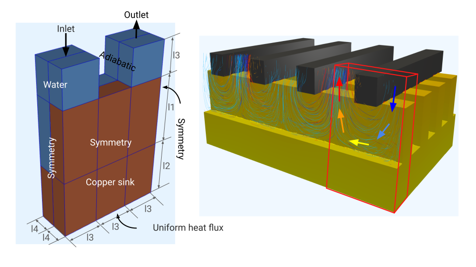
Simulation setup guide

Here you’ll find a simplified, example case level guide for setting up a conjugate heat transfer simulation in a microchannel heat sink.

Step 1 - Define variables

1. Start out in the Common sidebar by defining variables for model dimensions:

   Name	Description	Expression
   l1	length 1 [m]	0.6e-3
   l2	length 2 [m]	0.5e-3
   l3	length 3 [m]	0.3e-3
   l4	length 4 [m]	0.15e-3
   m1	Number of mesh segments along l1	12
   m2	Number of mesh segments along l2	10
   m3	Number of mesh segments along l3	12
   m4	Number of mesh segments along l4	5

2. Define variables for other key values:

   Name	Description	Expression
   VolumeFlowRate	Volume flow rate [mL/s]	0.0001
   UniformHeatFlux	Uniform heat flux [W/m^2]	220000
   InletArea	Area of inlet [m^2]	l3 * l3
   InletVel	Inlet velocity magnitude [m/s]	VolumeFlowRate * 1e-6 / InletArea
   InletTemp	Inlet temperature [K]	293
   Ahsbase	Base area for thermal resistance calculation [m^2]	10.02 * 11.4 * 1e-6

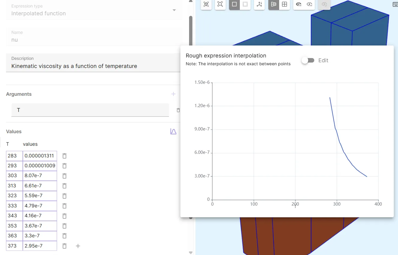
3. Define the interpolated function nu:

   Name	Description	Arguments
   nu	Kinematic viscosity as a function of temperature	T

   Import file viscosity.csv, containing the following 10 rows of input-value pairs for nu:

   T	values
   283	0.000001311
   293	0.000001009
   303	8.07e-7
   313	6.61e-7
   323	5.59e-7
   333	4.79e-7
   343	4.16e-7
   353	3.67e-7
   363	3.3e-7
   373	2.95e-7

Finalized nu:

Step 2 - Build the geometry

1. In the Model section, create the model geometry by building Box elements and using the Translation operation:

   Name	Element type	Center point [m]	Size [m]	Rotation [deg]
   box	Box	X: 0	X: l4	X: 0
   		Y: -l3	Y: l3	Y: 0
   		Z: l2 / 2	Z: l2	Z: 0

   Name	Element type	Target volumes	Translation [m]	Copy	Repeat count
   translate	Translation	first box	X: 0	☑️	2
   			Y: l3
   			Z: 0

   Name	Element type	Target volumes	Translation [m]	Copy	Repeat count
   translate 2	Translation	all three first-level boxes	X: -l4	☑️	1
   			Y: 0
   			Z: 0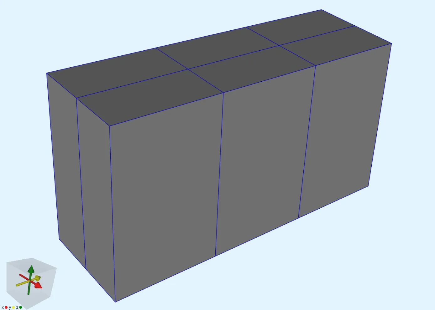

   

2. Continue adding elements:

   Name	Element type	Center point [m]	Size [m]	Rotation [deg]
   box 2	Box	X: 0	X: l4	X: 0
   		Y: -l3	Y: l3	Y: 0
   		Z: l1 / 2 + l2	Z: l1	Z: 0

   Name	Element type	Target volumes	Translation [m]	Copy	Repeat count
   translate 3	Translation	box 2	X: 0	☑️	2
   			Y: l3
   			Z: 0

   Name	Element type	Target volumes	Translation [m]	Copy	Repeat count
   translate 4	Translation	three second-level boxes	X: -l4	☑️	1
   			Y: 0
   			Z: 0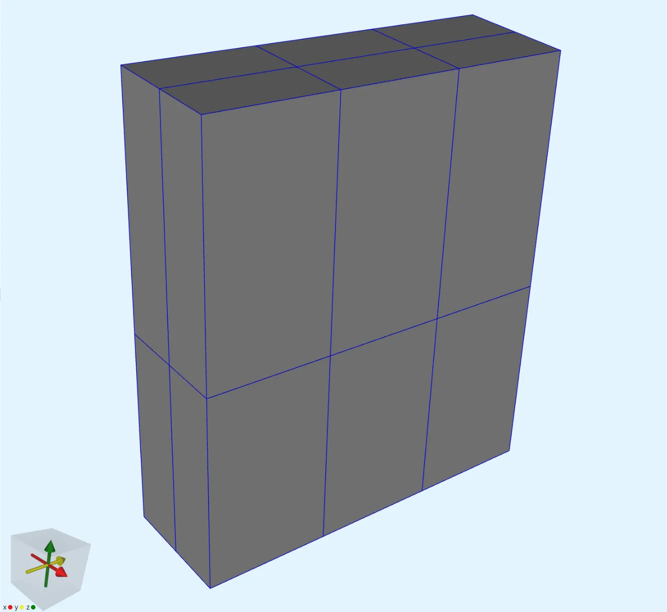

   

3. Add the remaining elements:

   Name	Element type	Center point [m]	Size [m]	Rotation [deg]
   box 3	Box	X: 0	X: l4	X: 0
   		Y: -l3	Y: l3	Y: 0
   		Z: l3 / 2 + l2 + l1	Z: l3	Z: 0

   Name	Element type	Target volumes	Translation [m]	Copy	Repeat count
   translate 5	Translation	box 3	X: -l4	☑️	1
   			Y: 0
   			Z: 0

   Name	Element type	Target volumes	Translation [m]	Copy	Repeat count
   translate 6	Translation	two third-level boxes	X: 0	☑️	1
   			Y: 2 * l3
   			Z: 0

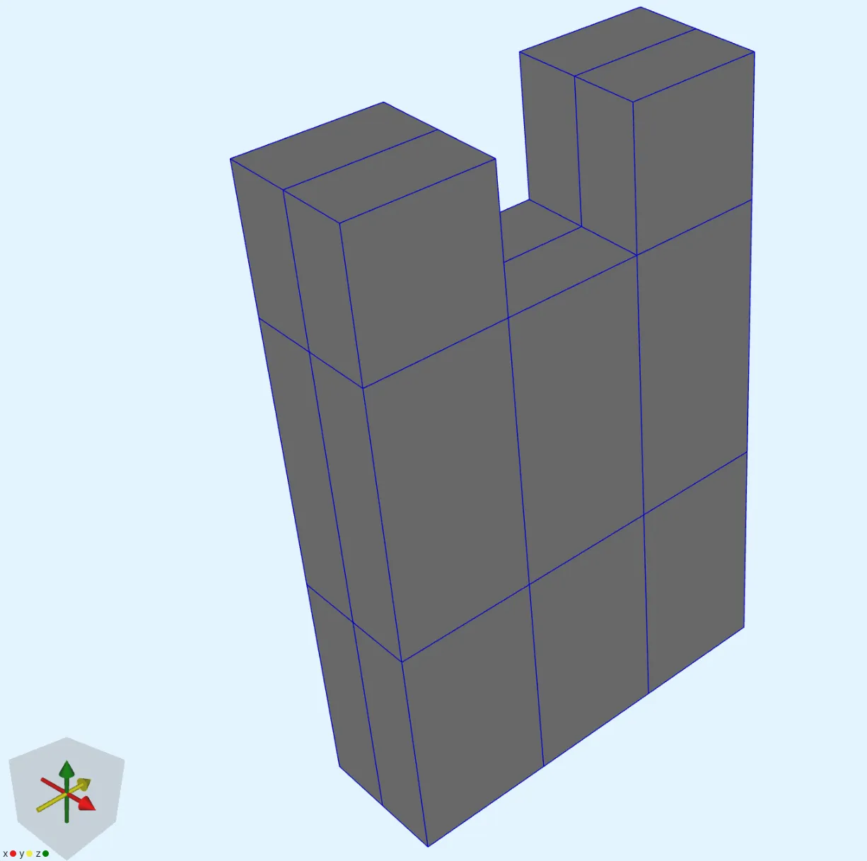
Finished geometry:

Step 3 - Define the materials

After confirming model changes, go to the Physics section to define model materials.

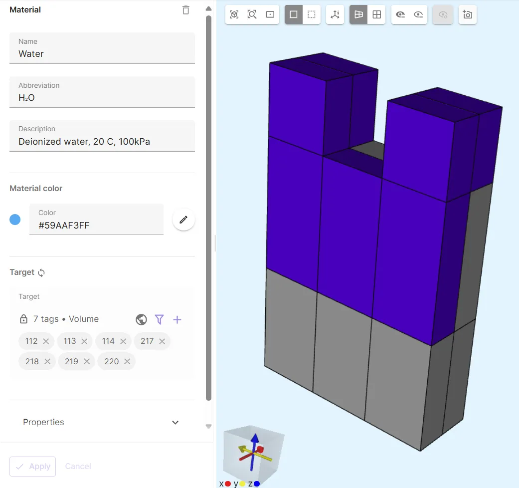
Material 1 - Water

Assign Water to the seven water box volumes (see image below).

Viscosity

In material properties, change the Dynamic viscosity of water to 998 * nu(T).

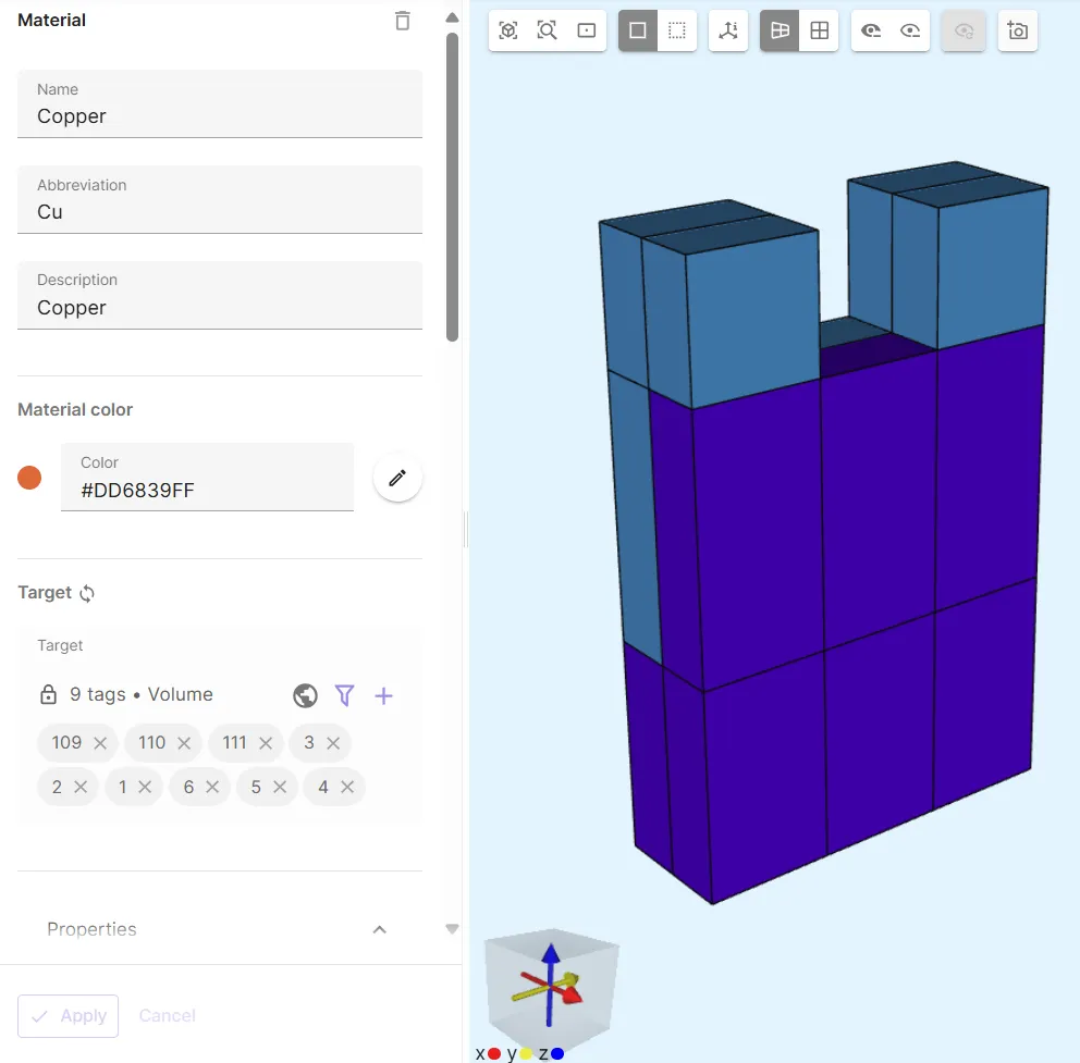
Material 2 - Copper

Assign Copper to the remaining copper box volumes.

Step 4 - Define the physics

Go to the Physics section.

The Laminar flow, Heat solid and Heat fluid physics are required for CHT. Add all of them before moving on to define interactions.

Physics 1 - Laminar flow

• As laminar flow target, select the water box volumes.

• Add Velocity constraint and name it as Inlet:

  Name	Interaction type	Target	Value
  Inlet	Velocity constraint	Inlet surfaces	[0; 0; -InletVel]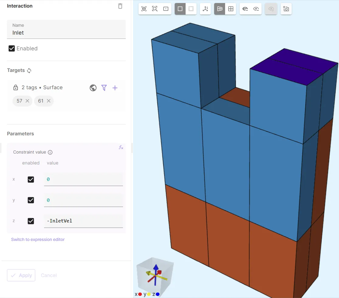

  

• Add Pressure constraint and name it as Outlet:

  Name	Interaction type	Target	Value
  Outlet	Pressure constraint	Outlet surfaces	0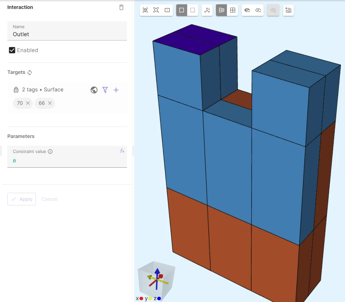

  

• Add Velocity constraint and name it as CHTWalls:

  Name	Interaction type	Target	Value
  CHTWalls	Velocity constraint	Water/copper boundary surfaces	[0; 0; 0]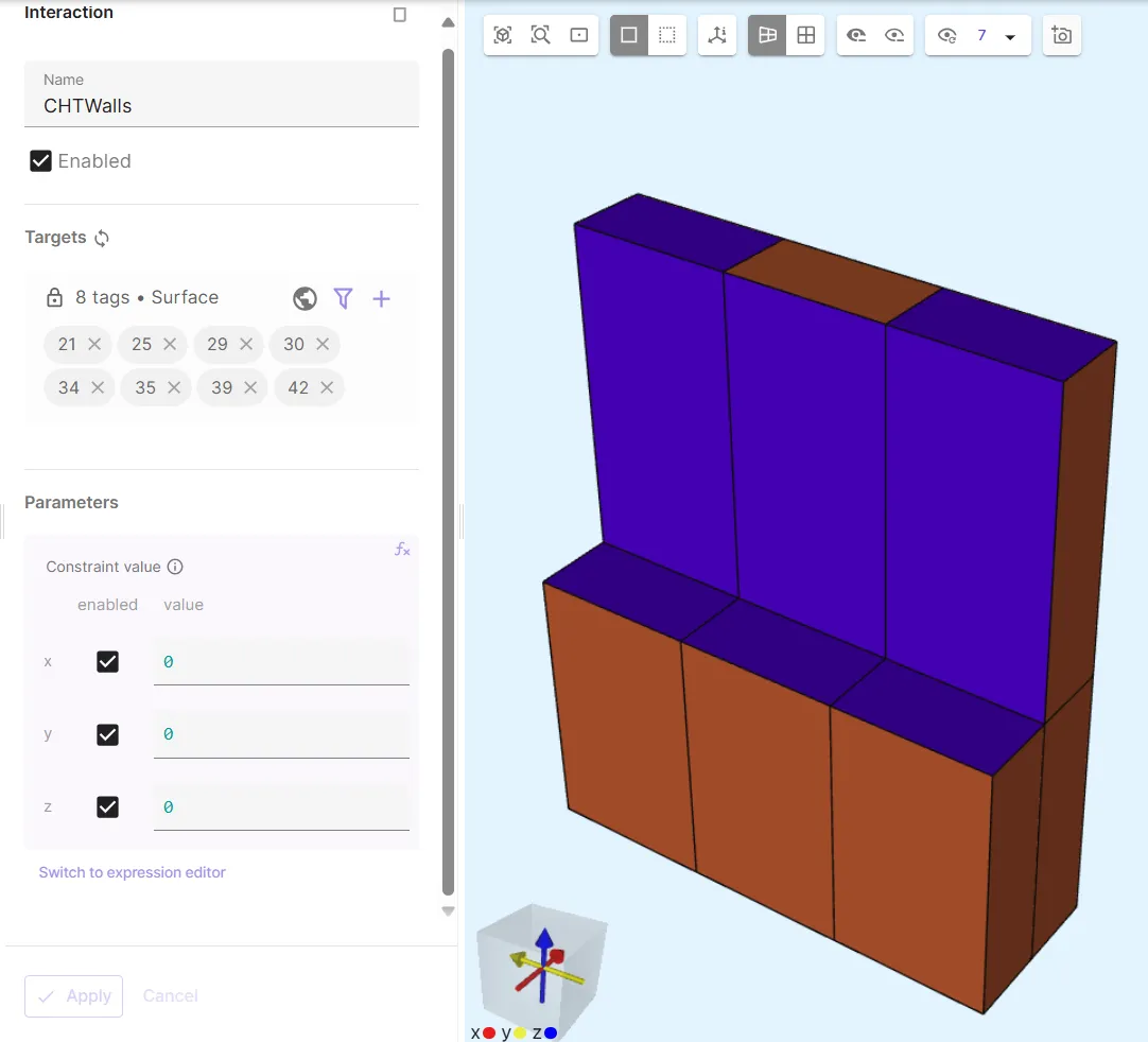

  

• Add Velocity constraint and name it as AdiabaticWater:

  Name	Interaction type	Target	Value
  AdiabaticWater	Velocity constraint	Water inner boundary surfaces	[0; 0; 0]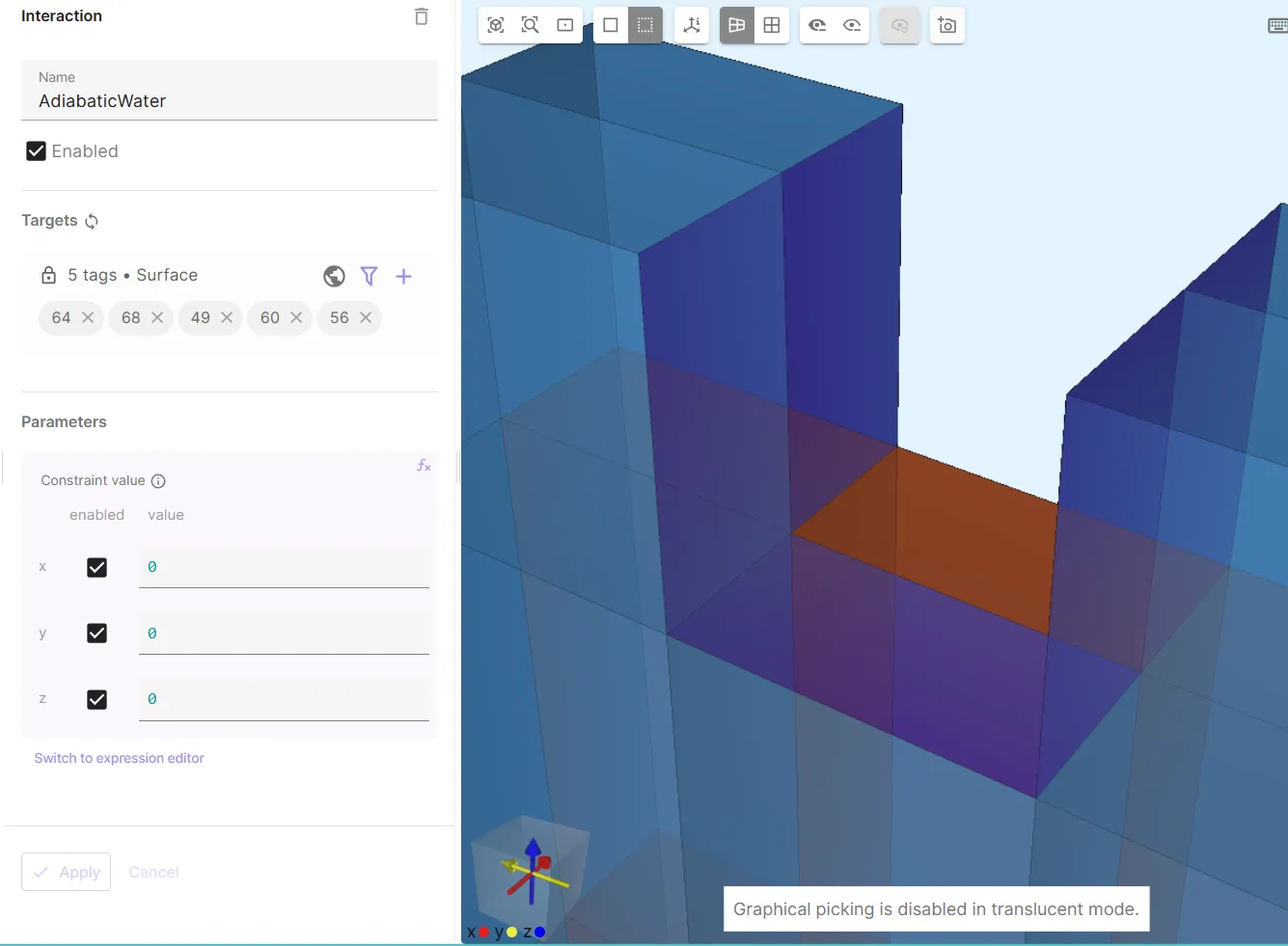

  

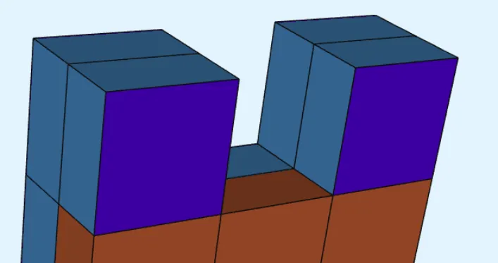
• Add Velocity symmetry and name it as SymmetryWallX:

  Name	Interaction type	Target
  SymmetryWallX	Velocity symmetry	Water boundary surfaces perpendicular to X-axis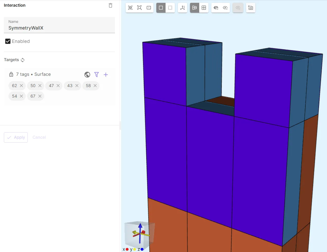

  

  Remember to also select the water boundaries on the backside:

  

• Add Velocity symmetry and name it as SymmetryWallY:

  Name	Interaction type	Target
  SymmetryWallY	Velocity symmetry	Water boundary surfaces perpendicular to Y-axis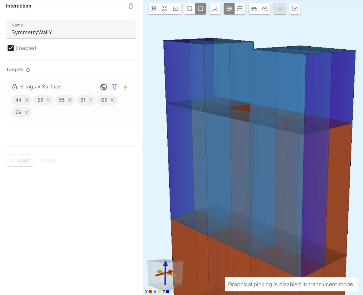

  

• Add Thermal fluid to couple Laminar flow with Heat fluid.

Physics 2 - Heat solid

• As Heat solid target, select all copper box volumes.

• Add Heat source and name it as UniformHeatFlux.

  Name	Interaction type	Target	Heat source
  UniformHeatFlux	Heat source	Copper bottom surfaces	UniformHeatFlux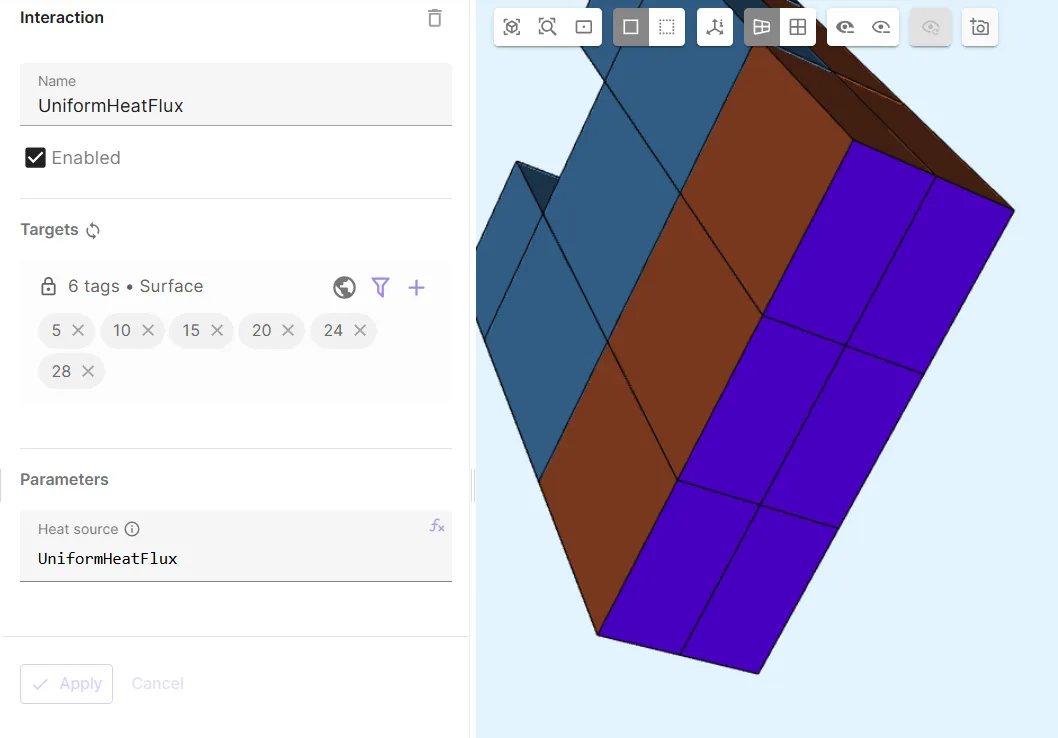

  

Physics 3 - Heat fluid

• As Heat fluid target, select the water region.

• Add Constraint and name it as Tinlet.

  Name	Interaction type	Target	Temperature constraint
  Tinlet	Constraint	Inlet surfaces	InletTemp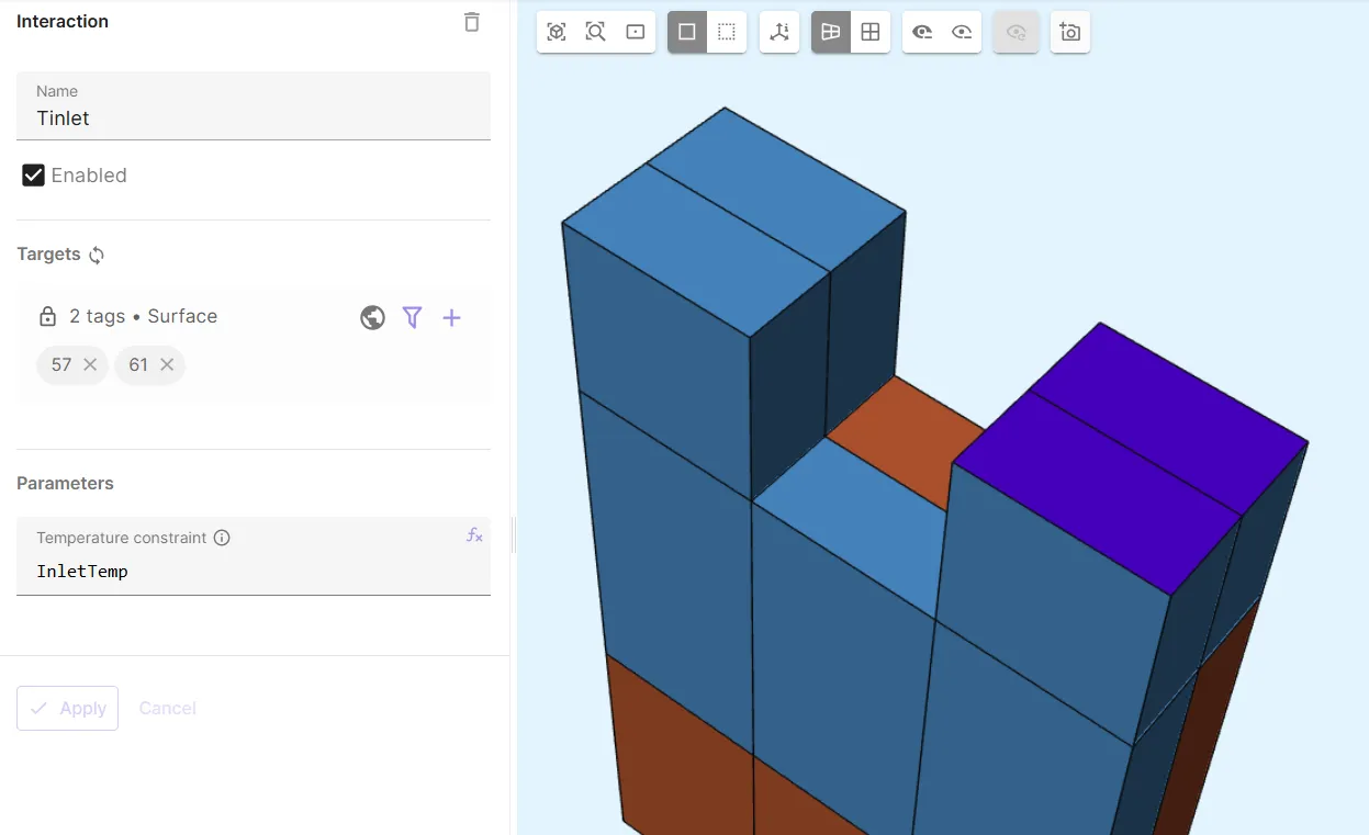

  

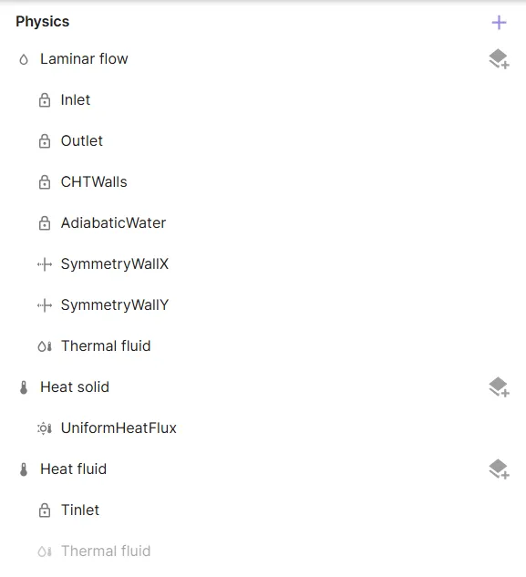
Your physics are now defined. Before moving on, check that your physics tree matches the one below.

Step 5 - Generate the mesh

Proceed to the Simulations section and create a new transfinite mesh:

1. Under Customizations, add transfinite mesh entities for each volume in the model, 16 in total.

2. Assign a unique volume as target for each entity, so that each volume is targeted once.

3. Apply the settings to save your work so far.

4. Assign lengths to your transfinite mesh entity segments according to this table:

   Transfinite mesh entities	Target volumes	A Segments	B Segments	C Segments
   1-6	Bottom layer boxes	m2 (5e-5)	m3 (2.5e-5)	m4 (3e-5)
   7-12	Middle layer boxes	m1 (5e-5)	m3 (2.5e-5)	m4 (3e-5)
   13-16	Top layer boxes	m3 (2.5e-5)	m3 (2.5e-5)	m4 (3e-5)

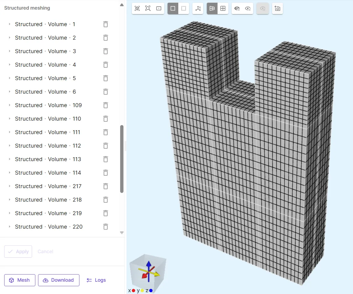
Finished mesh:

Step 6 - Simulate

In the Simulations section, create a new simulation:

• In Simulation settings:
  • Set Analysis type to Static.
  • Set Solver mode to Direct solver.
• As Mesh, select the mesh you created.
• There are plenty of available options for Outputs. Choose those interesting to you from the table below:

Output type	Name	Output expression
Field	p	p
Field	V	V
Field	T	T
Custom value	flowratein	integrate(reg.inlet_target, transpose(V)*-normal(reg.water_target),2)
Custom value	flowrateout	integrate(reg.outlet_target, transpose(V)*-normal(reg.water_target),2)
Custom value	AvgCHTWallTemp	integrate(reg.chtwalls_target, T, 2)/integrate(reg.chtwalls_target, 1.0, 2)
Custom value	PressureDrop	integrate(reg.inlet_target, p, 2)/integrate(reg.inlet_target, 1.0, 2)-integrate(reg.outlet_target, p, 2)/integrate(reg.outlet_target, 1.0, 2)
Custom value	Tbasemax	maxvalue(reg.uniformheatflux_target, T, 2)
Custom value	Tbasemin	minvalue(reg.uniformheatflux_target, T, 2)
Custom value	Tbaseavg	integrate(reg.uniformheatflux_target, T, 2)/integrate(reg.uniformheatflux_target, 1.0, 2)
Custom value	ThermalResistance	(maxvalue(reg.uniformheatflux_target, T, 2)-InletTemp)/(UniformHeatFlux*Ahsbase)
Custom value	PumpingPower	(integrate(reg.inlet_target, p, 2)/integrate(reg.inlet_target, 1.0, 2)-integrate(reg.outlet_target, p, 2)/integrate(reg.outlet_target, 1.0, 2))*abs(integrate(reg.inlet_target, transpose(V)*-normal(reg.water_target),2))
Custom value	MeanAbsoluteTemperatureDeviation	(abs(maxvalue(reg.uniformheatflux_target, T, 2) - integrate(reg.uniformheatflux_target, T, 2)/integrate(reg.uniformheatflux_target, 1.0, 2)) + abs(minvalue(reg.uniformheatflux_target, T, 2) - integrate(reg.uniformheatflux_target, T, 2)/integrate(reg.uniformheatflux_target, 1.0, 2)))/2.0

You can run the simulation after selecting options and outputs.

Step 7 - Results

In the Simulations section, you can add visualizations to see field output results. Some examples are given below.

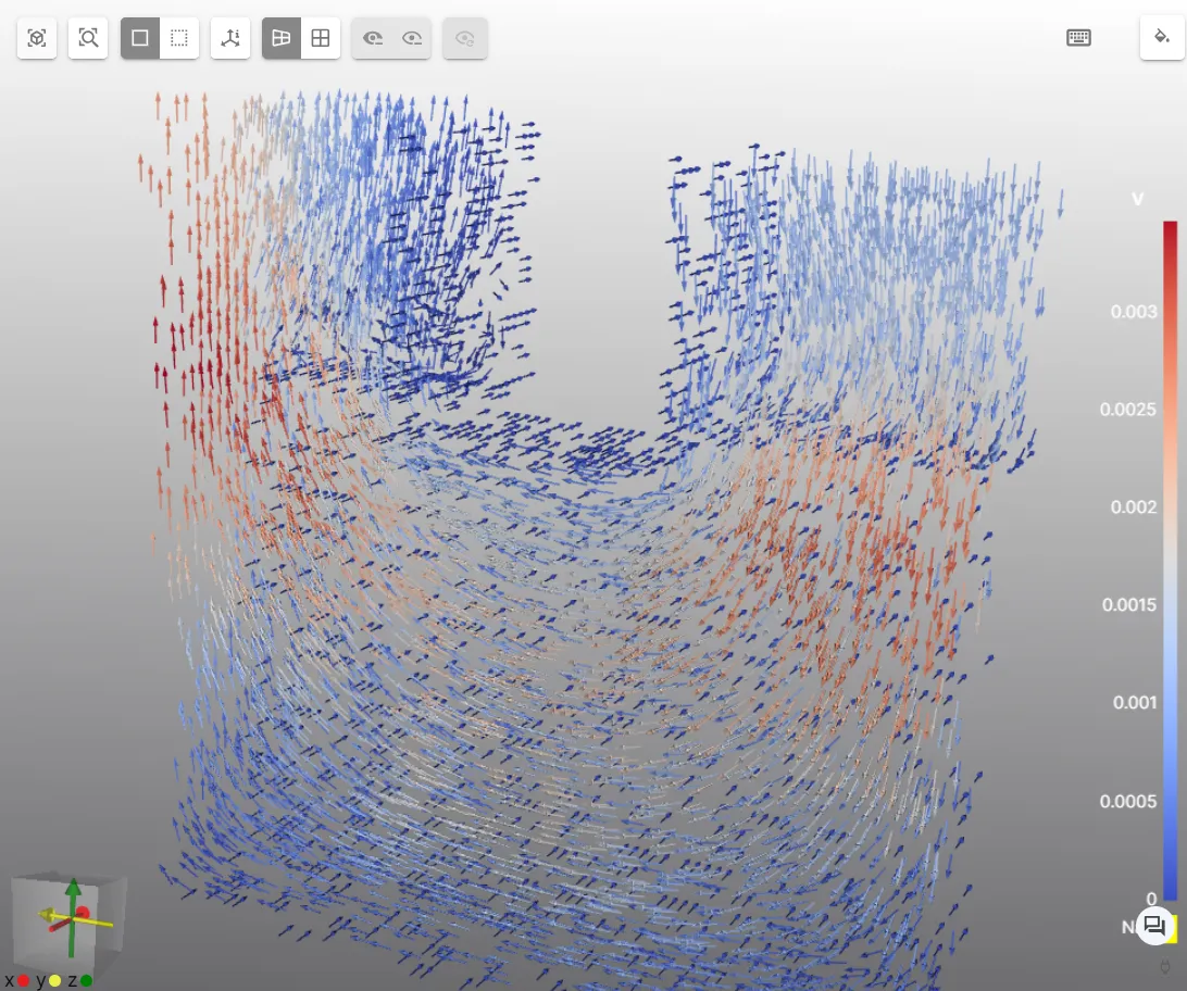
• Velocity field visualization:
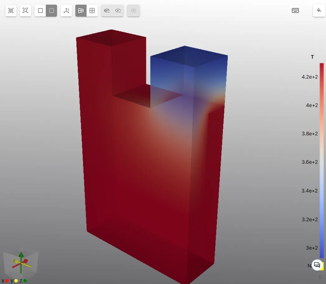
• Temperature field visualization:

In a static simulation, only one data point is extracted for each custom value output. You can see custom value output data in the Summary:

To extract multiple values for custom value outputs to create plots, use a sweep or a transient simulation with enough sweep/time-steps.

References

[1] K. Tang, G. Lin, Y. Guo, J. Huang, H. Zhang, J. Miao. Simulation and optimization of thermal performance in diverging/converging manifold microchannel heat sink. International Journal of Heat and Mass Transfer, Vol 200, 2023. https://doi.org/10.1016/j.ijheatmasstransfer.2022.123495.