Static heat transfer in solid materials - NAFEMS Benchmark

What you’ll learn

• How to create a box geometry and define regions for different boundary surfaces.
• How to create a custom material with specific thermal properties and set up Heat solid physics with constraint (Dirichlet) and heat source (convection) boundary conditions.
• How to use transfinite meshing for structured grids, add a custom interpolate output to probe temperature at a specific point, and modify the script to linearize a boundary source term for convergence.

In this tutorial, a NAFEMS benchmark test for thermal analysis is set up and simulated. ¹

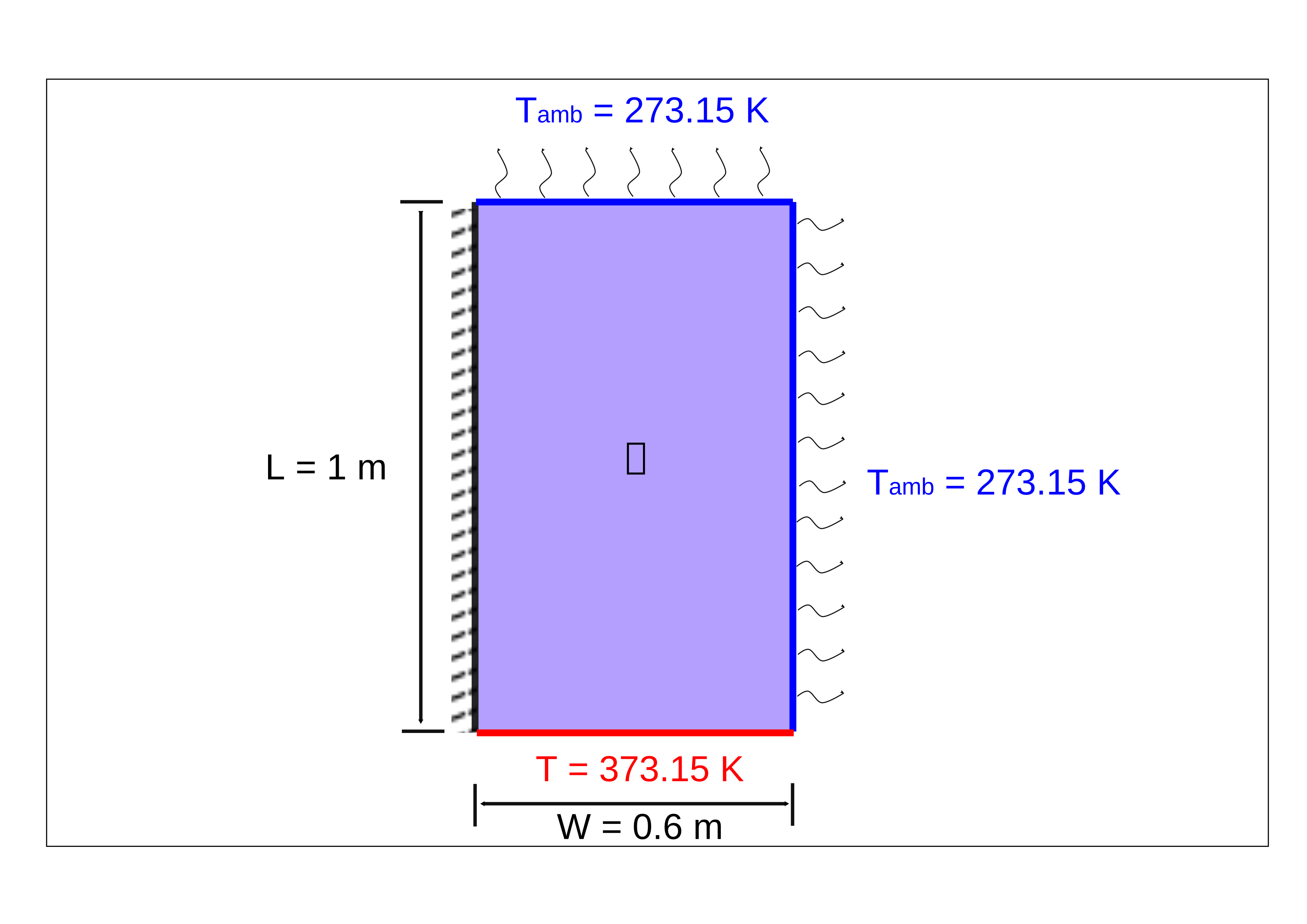
Model definition

A steady-state thermal analysis is performed with different boundary conditions (BCs) including adiabatic (insulated or zero heat flux), Dirichlet BCs, and finite heat flux by natural convection specified by a known heat transfer coefficient.

The result is a steady-state temperature distribution in the spatial domain. The image below shows the schematic of the spatial domain with BCs.

Output Results

• Temperature at coordinates $(0.3, -0.3, 0.0) \rm ~ m$, which is on the right boundary exposed to ambient. The benchmark value is $291.4 \rm ~ K$.

Material Data

Property	Value	Unit
Density	$1.0$	$\rm kg/m^3$
Specific heat capacity	$1.0$	$\rm J/(kg K)$
Thermal conductivity	$52.0$	$\rm W/(m K)$

Boundary conditions

Name	Type	Value	Unit
left boundary	heat flux	$0.0$	$\rm W/m^2$
bottom boundary	temperature	$373.15$	$\rm K$
right boundary	heat flux	$-h (T - T_{\rm amb}$)	$\rm W/m^2$
top boundary	heat flux	$-h (T - T_{\rm amb}$)	$\rm W/m^2$
ambient $(T_{\rm amb})$	temperature	$273.15$	$\rm K$
natural convection	heat transfer coefficient $(h)$	$750.0$	$\rm W/(m^2K)$
front boundary	heat flux	$0.0$	$\rm W/m^2$
back boundary	heat flux	$0.0$	$\rm W/m^2$

Step-by-step guide

Here you’ll find a detailed step-by-step tutorial on how to set up a NAFEMS thermal analysis simulation in Quanscient Allsolve.

Step 1 - Build the geometry

1. Create a new project and name it as

   NAFEMS 2D Heat Transfer Benchmark

2. Start off with a box element.

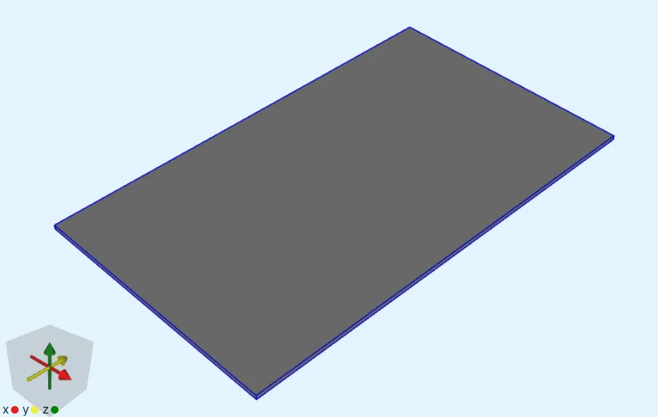
3. Edit the size of the box:

   Name	Element type	Center point [m]	Size [m]	Rotation [deg]
   box	Box	X: 0	X: 0.6	X: 0
   		Y: 0	Y: 1.0	Y: 0
   		Z: 0	Z: 0.01	Z: 0

Step 2 - Define regions

1. Proceed to the Common sidebar.

2. Define regions:

   Region name	Region type	Target
   ConstantTemperature	Surface	Y bottom surface
   NaturalConvection	Surface	X and Y top surfaces

Step 3 - Define the material

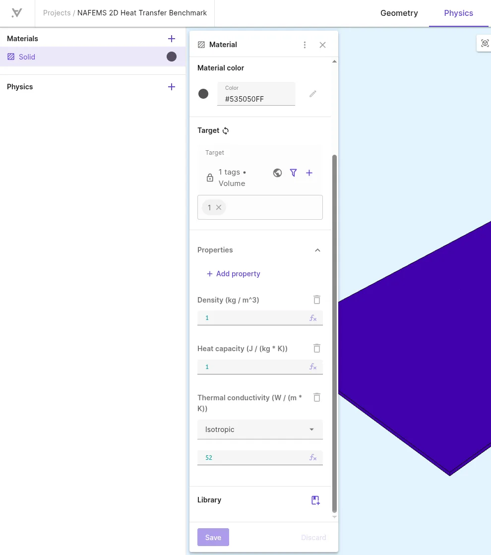
1. Create a new material in the Physics section:

   Name	Abbreviation	Description	Color	Target
   Solid		NAFEMS material	Dark grey	Box volume

2. Add properties to the material:

   Property	Value
   Density	1
   Heat capacity	1
   Thermal conductivity	52

Step 4 - Define variables

Define variables:

Name	Description	Expression
h	Heat transfer coefficient (W/m^2/K)	750
Tamb	Ambient temperature (K)	273.15

Step 5 - Define physics and boundary conditions

1. Go to the Physics section.

2. Add the Heat solid physics.

   Physics	Target
   Heat solid	Box volume

3. Add a Constraint interaction to Heat solid:

   Name	Interaction type	Target	Value
   Constraint	Constraint	ConstantTemperature region	375.15

4. Add a Heat source interaction to Heat solid:

   Name	Interaction type	Target	Value
   Heat source	Heat source	NaturalConvection region	-h * (T - Tamb)

Note: Zero heat flux

In the finite element formulation of Quanscient Allsolve, the zero heat flux (zero Neumann) boundary condition is automatically applied. There is no need to set it up manually.

Step 6 - Generate the mesh

1. Go to the Simulations section.

2. Create a new mesh.

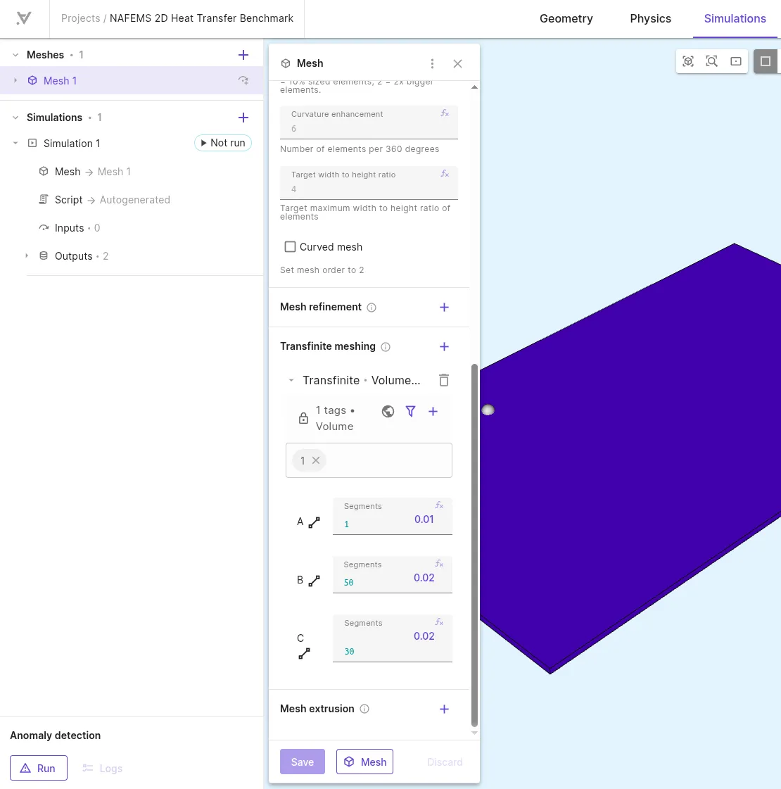
3. Under Customizations, add a Transfinite meshing entity of type Volume:

4. Select the box volume as the structured mesh entity target.

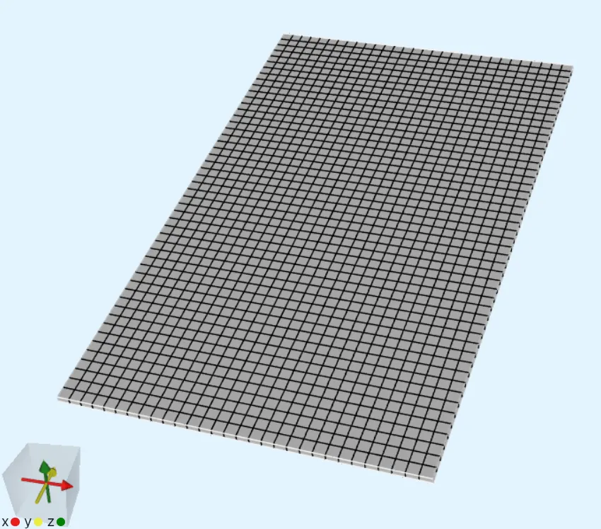
   Structured mesh entity type	Target	Segments
   Volume	box volume	A: 50
   		B: 1
   		C: 30

   Segment directions

   The segment directions (A, B, C) correspond to different edge curves on the model. Verify the assignment by checking the mesh preview: only 1 element should exist in the Z-direction (the thin direction) to mimic a 2D domain, while the X- and Y-directions should have finer subdivision.

   With these options, only one element is created in the Z-direction to mimic a 2-dimensional domain. Elements of length $0.02 ~ \rm m$ are created in the X- and Y-directions.

   

5. Generate the mesh and check the preview.

Step 7 - Apply simulation settings

1. Add a new simulation.

2. Set Analysis type to Static.

3. Select the mesh you created in Step 6 as the mesh for your simulation.

4. Add a T temperature field output.

5. Add a custom value output, which interpolates temperature at coordinates $(0.3, -0.3, 0.0) ~ \rm m$:

   Name	Output expression
   ProbeTemperature	interpolate(reg.solid_target, T, [0.3, -0.3, 0])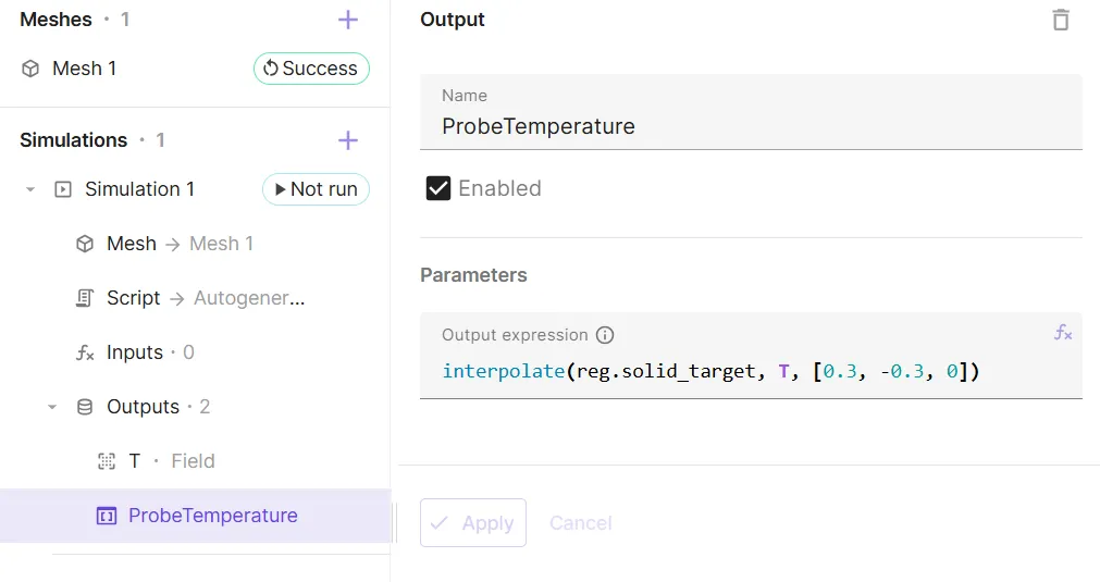

   

   Tip: Hover-over documentation

   When you hover over a function call, such as interpolate, the usage of the function is displayed in a documentation excerpt.

6. Run the simulation.

7. To check the progress of the simulation, check the Logs.

8. The relative change is increasing with each iteration, so the simulation will not converge. Abort the simulation.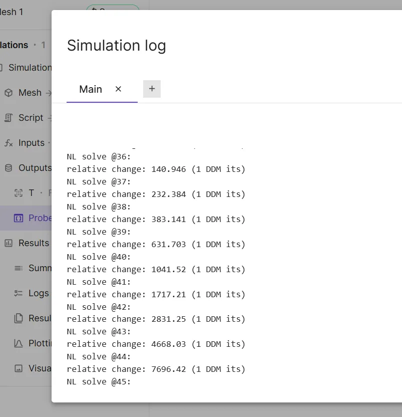

Step 8 - Edit the script

To solve the convergence issue, the Script needs some modification.

1. Open the Script and toggle on Scripting mode.

2. Change fld.T in the Heat source interaction formulation to qs.dof(fld.T). Save the script.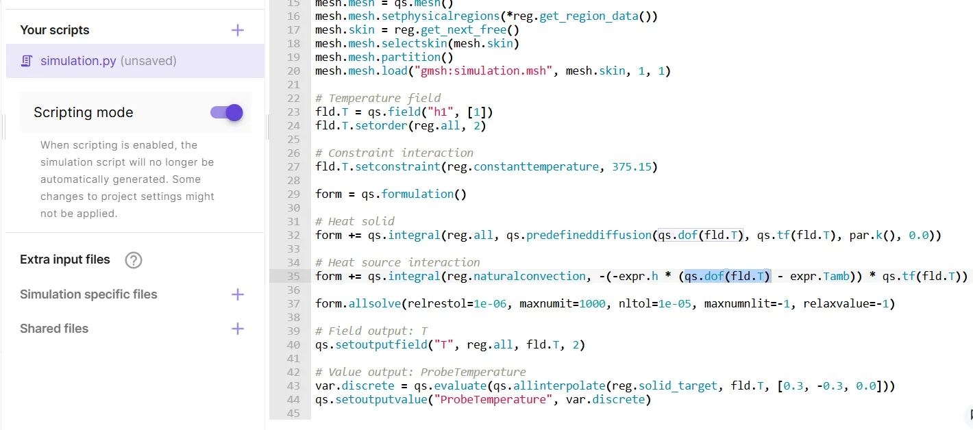

   

   Note: Script modification

   This modification in the script changes the temperature field to an unknown, which is solved during iterations.

   The idea is to linearize the boundary source term, which in turn makes the diagonal of the assembly matrix dominant, resulting in a well-conditioned problem that will converge.

3. Run the simulation again.

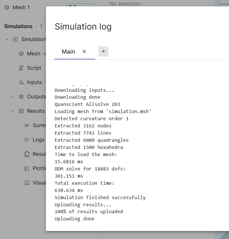
This time the simulation converges within one iteration as seen from the Logs.

Step 9 - See results

1. Add a visualization for the T field and render it. The steady-state temperature field distribution becomes visible.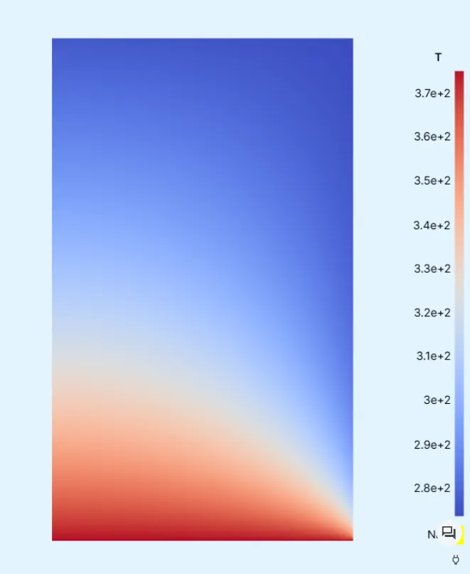

   

2. To check the ProbeTemperature value, check the Summary. Temperature at the probe location (0.3, -0.3, 0.0) m is 291.77 K, which is very close to the benchmark value¹ of 291.4 K.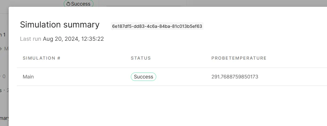

   

   Result accuracy scales with mesh density. An even more accurate result would be obtained with a finer mesh.

References

Footnotes

1. A.D. Cameron, J.A. Casey, G.B. Simpson. Benchmark Tests for Thermal Analysis. NAFEMS Documentation. ↩ ↩²