Permanent magnet synchronous electric motor

What you’ll learn

• How to import a STEP geometry, apply a translate operation to separate rotor and stator, and use regions for the rotating domain and air gap.
• How to set up Magnetism φ with remanence, rotational periodicity (antiperiodic), continuity conditions across the rotor-stator interface, and Lump I/V cut current sources on windings.
• How to modify the simulation script to move the rotor back into position, apply rotation, and compute torque via Arkkio’s method and the Maxwell stress tensor.

In this tutorial, a 3D permanent magnet synchronous electric motor is considered under magnetostatic conditions using the φ-formulation.

Model definition

Instead of the whole motor, only a 1/8 slice of the motor is modeled. The 1/8 slice functions as a symmetry cell, which can be set up to simulate the whole motor with symmetry conditions. The symmetry cell has its periodic face aligned with the X-axis.

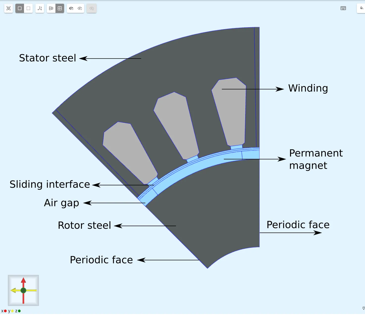
Element	Dimensions [m]
Stator steel outer radius	$0.100$
Stator steel inner radius	$0.059$
Rotor steel outer radius	$0.055$
Rotor steel inner radius	$0.025$
Permanent magnet outer radius	$0.058$
Air gap thickness	$0.001$

Material Data

• Linear steel

Property	Value
Magnetic permeability	$2000 \times \mu_0 = 2000 \times 4 \pi \times 10 ^{-7} ~ \rm H/m$

Boundary conditions

Name	Type	Value
left and right Y-planes	periodicity: rotation	antiperiodic
rotor-stator interface	continuity	potential equality on both sides

Output Results

• Torque [Nm]

Step-by-step guide

Here you’ll find a detailed step-by-step tutorial on how to simulate a permanent magnet synchronous electric motor in Quanscient Allsolve.

Step 1 - Build the geometry

1. Start with a new project and name it PMSM Electric motor.

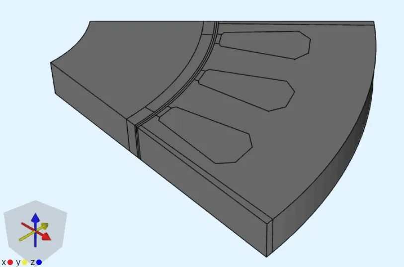
2. Import the STEP file containing the motor slice geometry. File download link: pmsm-electric-motor.step

   

3. Add a Translate operation to move the rotor up in the Z-direction. Find it by clicking + next to Geometry elements in the left sidebar and selecting Translate under Simple operation.

   Name	Element type	Target	Translation [m]	Copy
   translate	Translate operation	Rotor volumes	X: 0	No
   			Y: 0
   			Z: 0.02

   The Translate operation is done in this tutorial to separate the rotor and stator for meshing, and to have a duplicate mesh on the rotor-stator interface.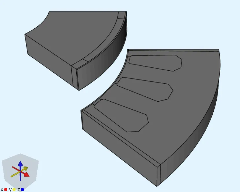

   

   The rotor is moved back into place at simulation time.

Caution: Position of geometry

In modelling a symmetry cell of a motor that has periodic boundaries:

1. The position of the geometry needs to be such that the rotation happens around the Z-axis.
2. One of the periodic boundaries needs to be aligned with the X-axis.

Step 2 - Define variables, materials and regions

1. Go to the Common sidebar.

2. Define variables:

   Name	Description	Expression
   I	Current amplitude [A]	300
   alpha	Mechanical angle [deg]	27
   phase	Electrical angle [deg]	0

3. Go to the Physics section to add materials. Add the Air material:

   Material	Target
   Air	permanent magnet domain and all air domains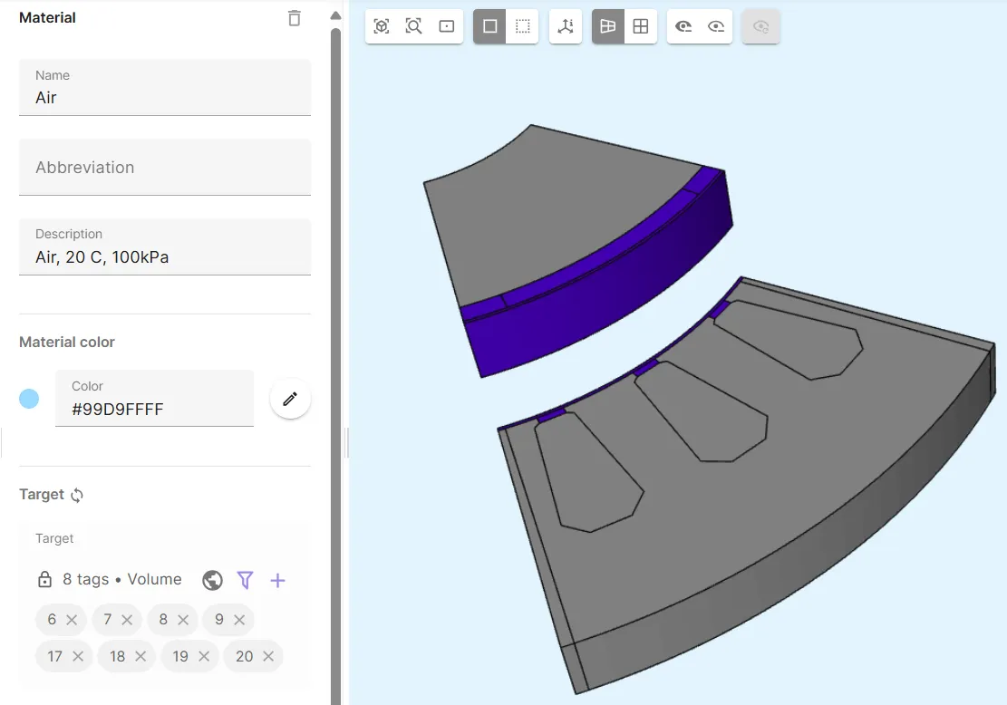

   

4. Add the Carbon steel AISI 1020 material:

   Material	Target
   Carbon steel AISI 1020	steel domain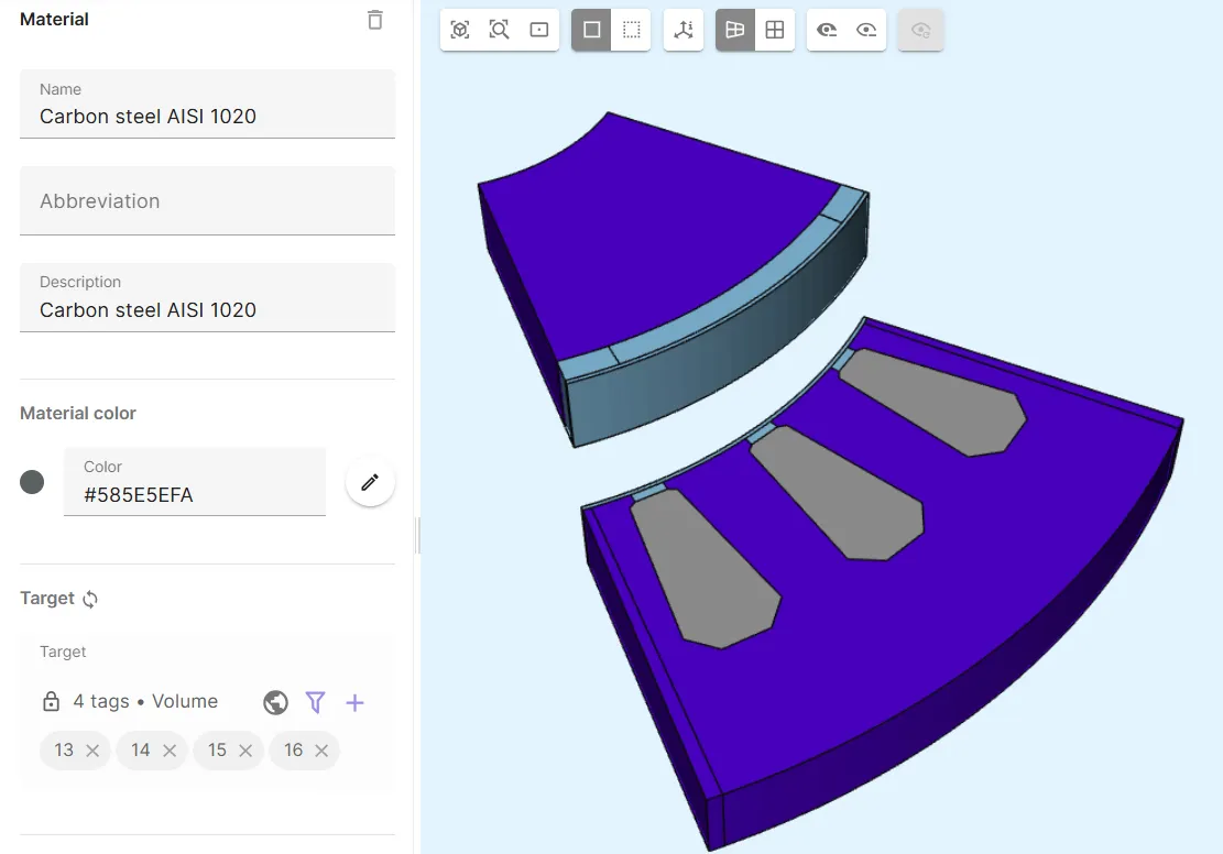

   

5. Instead of nonlinear permeability, linear permeability is applied to the steel in this tutorial. Edit Carbon steel AISI 1020 material properties:

   Property	Updated value
   Magnetic permeability	2000 * mu0

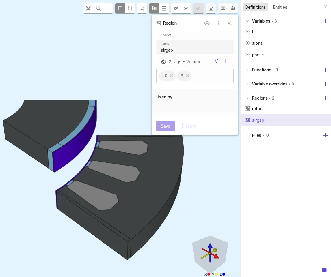
6. Define regions:

   Region name	Region type	Target
   rotor	Volume	all rotating regions with half of the airgap
   airgap	Volume	air gap between rotor and stator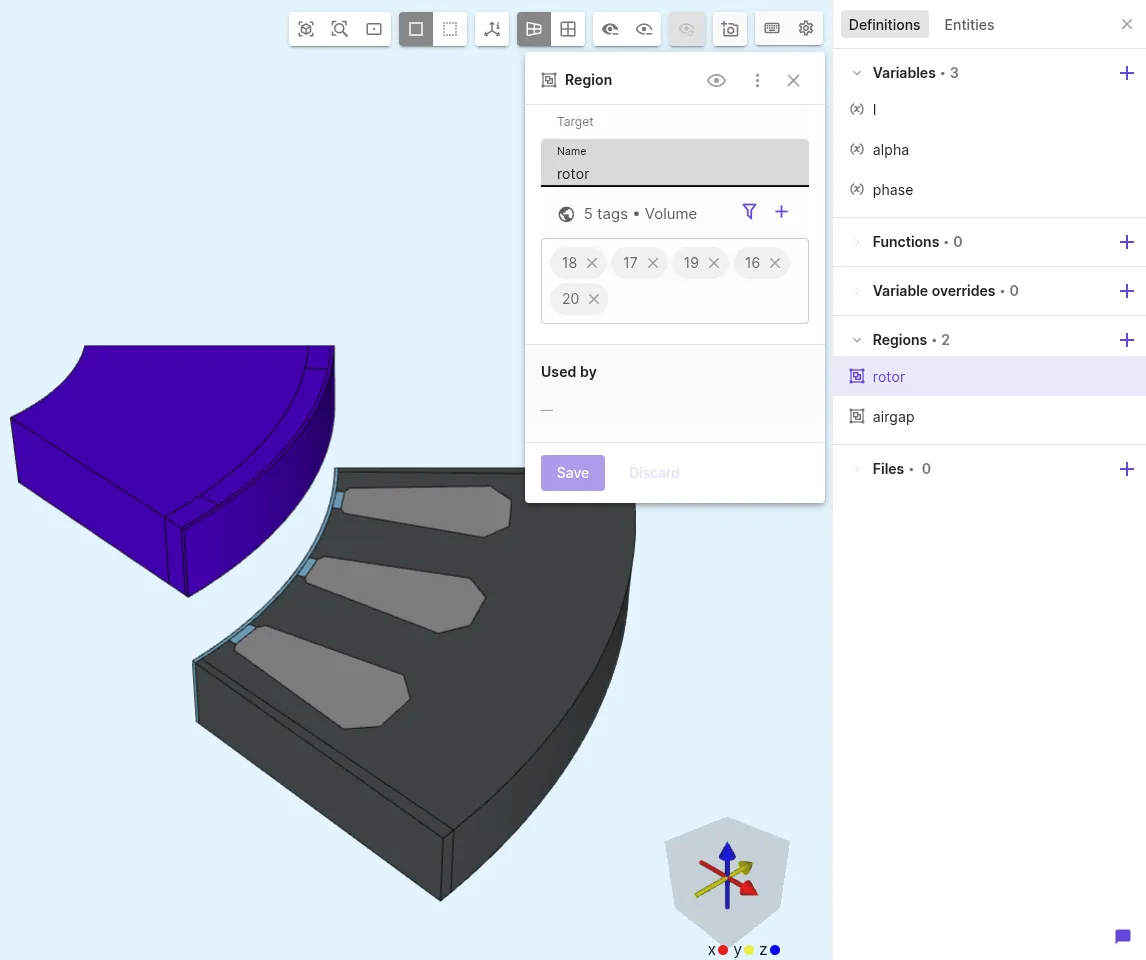

   

   

Step 3 - Define the physics and apply boundary conditions

1. Go to the Physics section.

2. Add the Magnetism φ physics:

   Physics	Target
   Magnetism φ	All volumes except the windings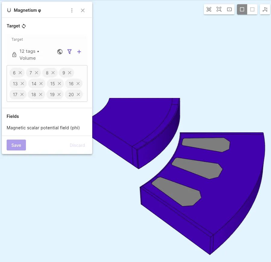

   

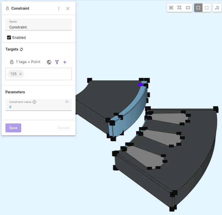
3. Add a Constraint interaction to Magnetism φ:

   Name	Interaction type	Target	Value
   Constraint	Constraint	a corner point on the permanent magnet	0

   This constraint is the gauge condition for the scalar potential φ. It will guarantee the uniqueness of the solution.

   

   Caution: Magnetism φ gauge condition target point

   Choose a target point on the Magnetism φ region so that it is not on the periodic boundaries nor on the sliding interface. E.g. the corner point of the permanent magnet in the air gap is a good option.

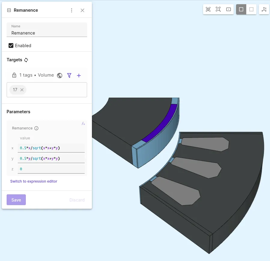
4. Add a Remanence interaction to Magnetism φ:

   Interaction name	Interaction type	Target	Value [X; Y; Z]
   Remanence	Remanence	Permanent magnet volume	[0.5*x/sqrt(x*x+y*y); 0.5*y/sqrt(x*x+y*y); 0]

   This introduces a $0.5 ~ \rm T$ radial magnetization to the motor.

   

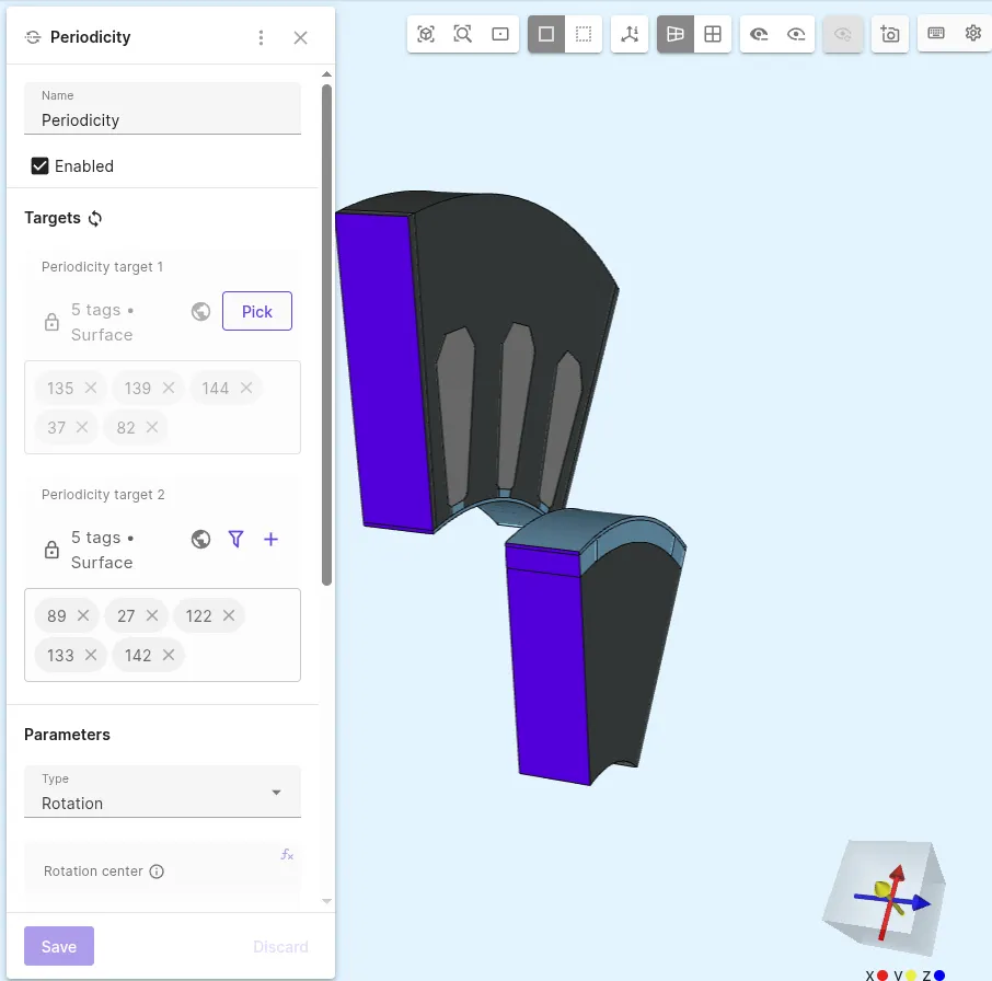
5. Add a Periodicity interaction and select target surfaces:

   Interaction name	Interaction type	Periodicity target 1	Periodicity target 2
   Periodicity	Periodicity	Side surfaces parallel to X-axis	Side surfaces opposite to target 1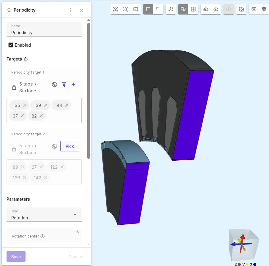

   

   

   Caution: Rotational periodicity and X-axis alignment

   When applying rotational periodicity, the first periodic surface needs to be aligned with the X-axis.

6. Select remaining options in the Periodicity interaction:

   Interaction name	Interaction type	Type	Rotation center [X; Y; Z]	Rotation angle [X; Y; Z]	Antiperiodicity
   Periodicity	Periodicity	Rotation	[0; 0; 0]	[0; 0; 45]	Yes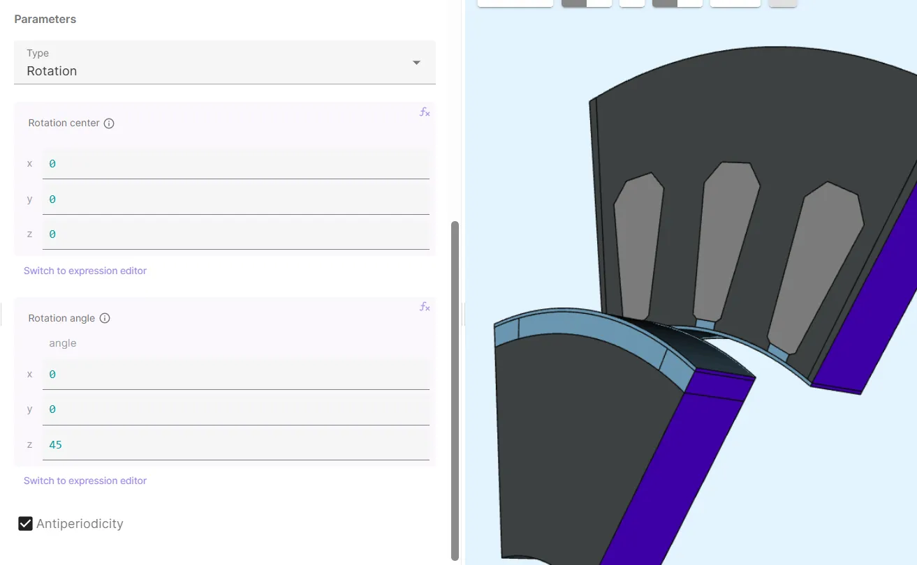

   

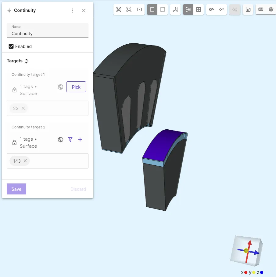
7. Add a Continuity interaction:

   Interaction name	Interaction type	Continuity target 1	Continuity target 2
   Continuity	Continuity	Stator interface surface	Rotor interface surface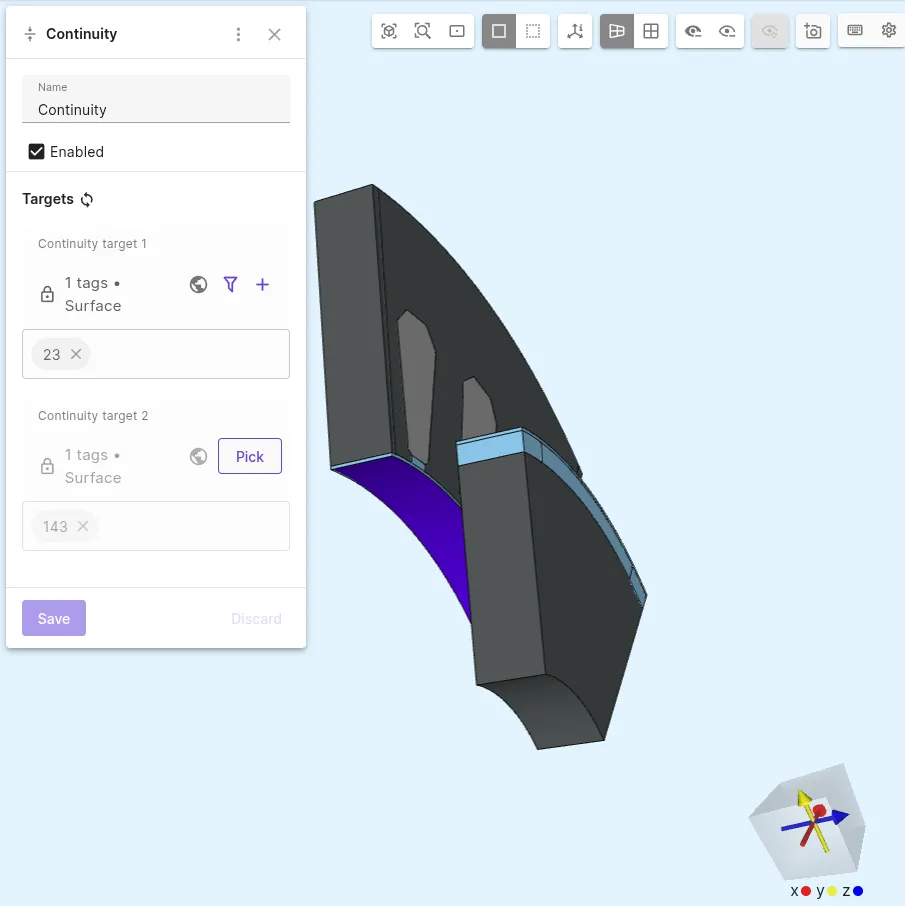

   

   

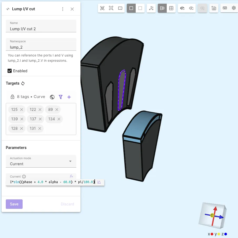
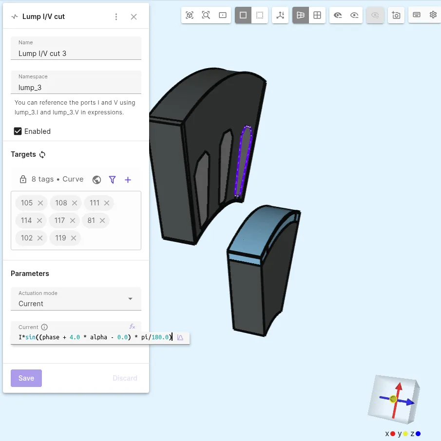
8. Add Lump I/V cut interactions to introduce current sources on the windings:

   Interaction name	Interaction type	Target	Actuation mode	Current
   Lump I/V cut	Lump I/V cut	Counterclockwise loop around left-most winding	Current	I * sin((phase + 4.0 * alpha - 120.0) * pi/180.0)
   Lump I/V cut 2	Lump I/V cut	Counterclockwise loop around middle winding	Current	I * sin((phase + 4.0 * alpha - 60.0) * pi/180.0)
   Lump I/V cut 3	Lump I/V cut	Counterclockwise loop around right-most winding	Current	I * sin((phase + 4.0 * alpha - 0.0) * pi/180.0)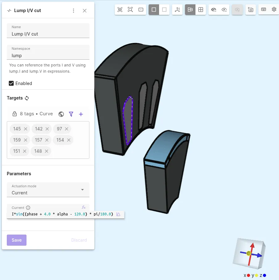

   

   

   

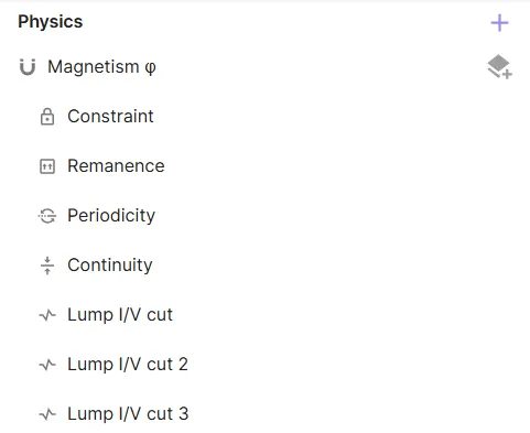
   Note: Electrical angle

   Here, the rotor has 8 poles. Therefore, the electrical angle is 8/2 times the mechanical angle at a synchronous speed.

There are 7 interactions in total:

Step 4 - Generate the mesh

1. Go to the Simulations section.

2. Create a new mesh.

3. Open the collapsible menu for Mesh element size.

4. Set mesh element max size to 0.001. Make sure you are using absolute size — if the relative size option is enabled, switch to absolute.

5. Enable Curved mesh.

6. Under Customizations, add a Mesh refinement entity:

   Mesh refinement entity type	Target	Max size
   Volume	air gap volumes	0.0005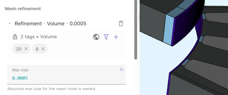

   

7. Apply settings and generate the mesh.

8. Select Default mesh to open a mesh preview in the model view.

   

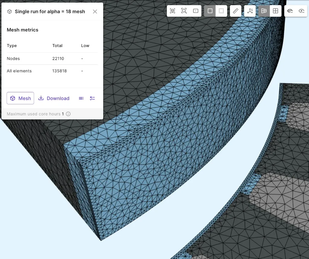
Step 5 - Apply simulation settings

1. Create a new simulation.

2. Set Analysis type to Static.

3. Select Mesh 1 as the mesh for your simulation.

4. Add a magnetic flux density B field output. As target, select all volumes except the windings.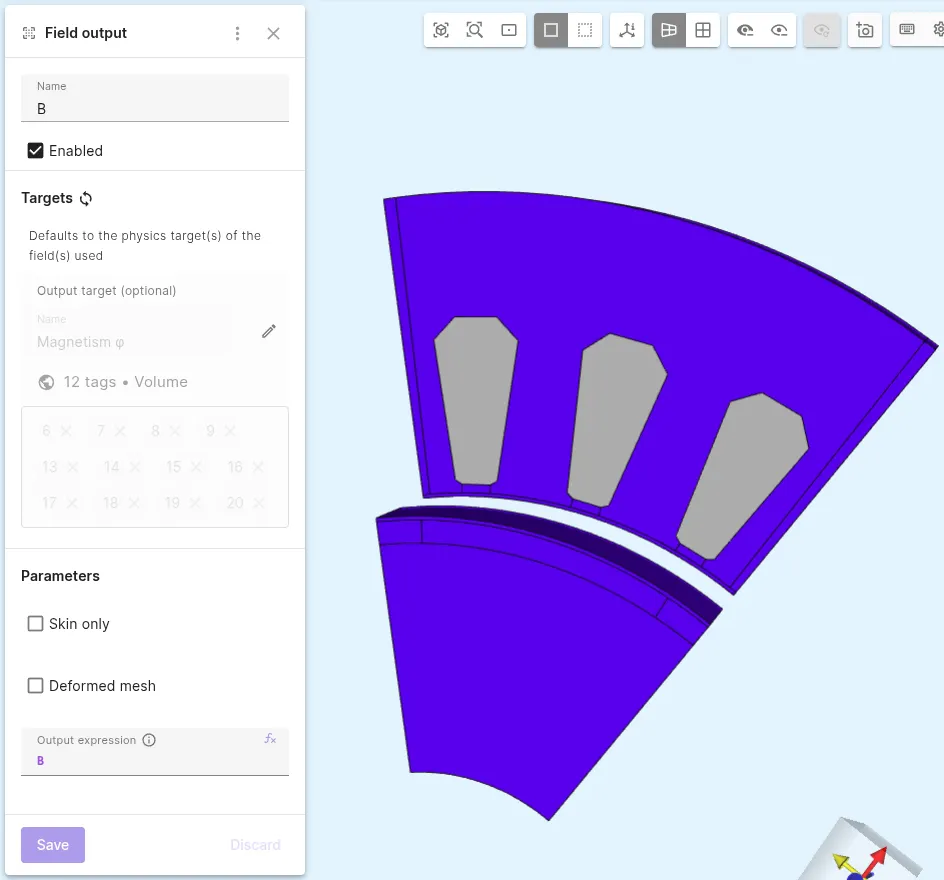

   

Step 6 - Modify the script

The following modifications need to be done by scripting:

• Move the rotor back to its original position and apply rotation.
• Apply antioperiodicity and rotation for the continuity condition.
• Calculate the torque.

To do these modifications, do the following:

1. Open the script for your simulation.

2. Enable scripting mode.

3. Add these lines to the script right below the initial mesh loading stage:

   # Moving the rotor back to it's original position and applying rotation
   mesh.mesh.shift(reg.rotor, 0.0, 0.0, -0.02)
   mesh.mesh.rotate(reg.rotor, 0.0, 0.0, expr.alpha)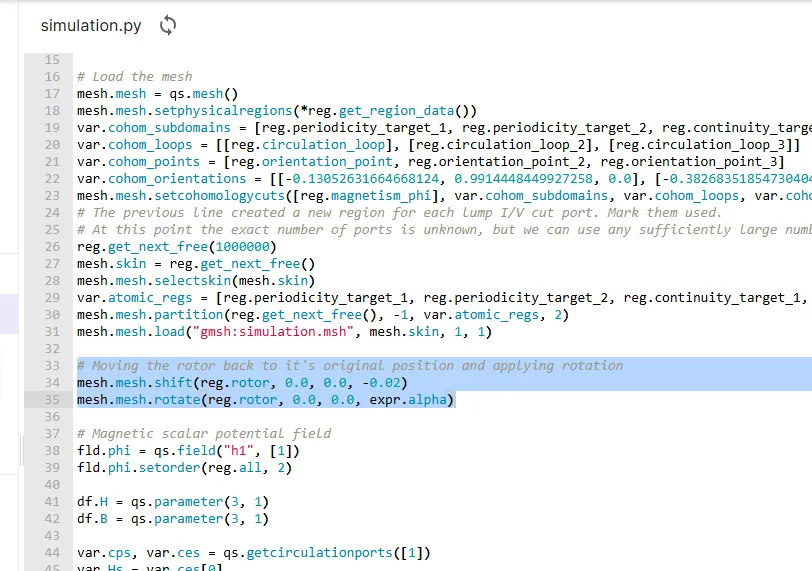

   

4. To address the antiperiodicity regarding the rotated position for the continuity condition, add the following arguments on the continuitycondition() function:

   qs.continuitycondition(..., [0,0,0], expr.alpha, 45.0, -1.0)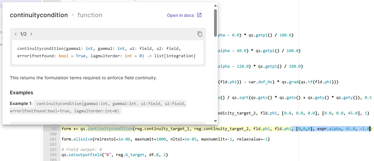

   

5. To calculate the torque via Arkkio’s method ¹ and via Maxwell’s Stress Tensor, add the following lines to the very end of the script:

   # Calculating torque:
   
   # The torque is scaled (8*5) to the actual z length of the motor 0.05 m and to take into account full 360 degrees of the motor.
   
   # 1) Using Arkkio's method
   rs = 0.059 # outer radius of airgap
   rr = 0.058 # inner radius of airgap
   radius = qs.sqrt( qs.pow(qs.getx(),2) + qs.pow(qs.gety(),2) )
   ephi = qs.array3x1(-qs.gety()/radius, qs.getx()/radius, 0.0)
   er = qs.array3x1(qs.getx()/radius, qs.gety()/radius, 0.0)
   Bphi = df.B*ephi
   Br = df.B*er
   dr = (rs-rr)
   magforcedensity1 = (8*5*radius*Br*Bphi/qs.getmu0()/dr)
   torque1 = magforcedensity1.allintegrate(reg.airgap,5)
   
   # 2) Using Maxwell stress tensor
   leverarm = qs.array3x1(qs.getx(), qs.gety(), 0.0)
   T = 1/qs.getmu0() * ( df.B*qs.transpose(df.B) - 0.5*df.B*df.B * qs.eye(3) )
   magforcedensity2 = qs.on(reg.airgap, T)*qs.normal(reg.airgap)
   torque2 = 8*5*qs.compz(qs.crossproduct(leverarm, magforcedensity2)).allintegrate(reg.continuity_target_2, 5)
   
   qs.setoutputvalue("Mechanical angle", qs.evaluate(expr.alpha)[0])
   qs.setoutputvalue("Torque (Arkkio)", qs.evaluate(torque1))
   qs.setoutputvalue("Torque (Maxwell's Stress Tensor)", qs.evaluate(torque2))

6. Save the script.

Step 7 - Running the simulation and checking results

1. Run Simulation 1.

2. To follow the simulation progress, open the Logs.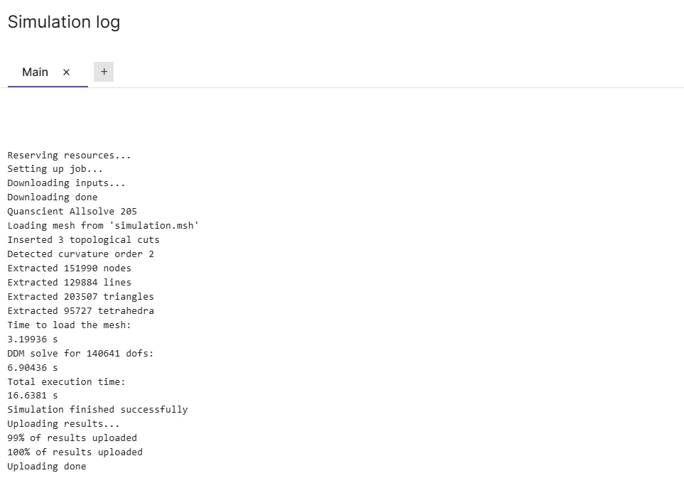

   

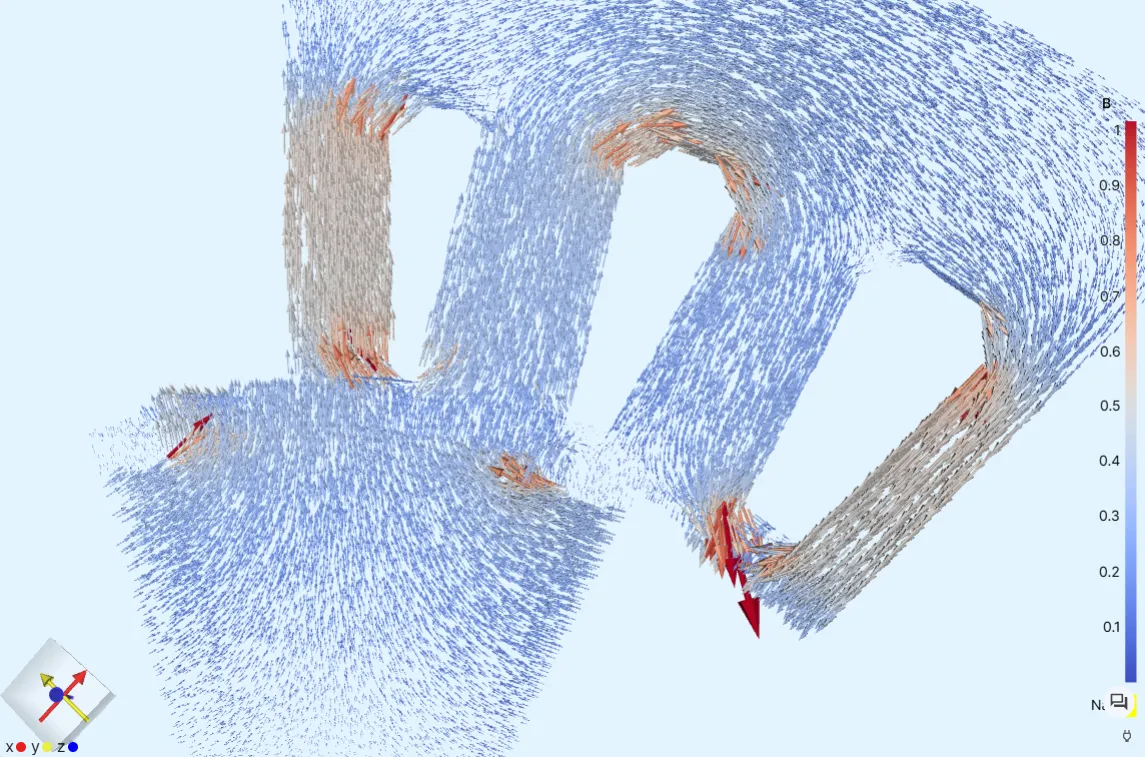
3. Once the simulation has finished, add a B field visualization.

4. Add a Glyph filter to the visualization:

   Filter	Layer	Max sample points	Scaling mode	Scale factor
   Glyph	B - Cool to Warm	50000	data	0.005
   	0.0002 - 1.0

5. Activate the visualization.

   

6. To see the value of torque [Nm] at the applied mechanical angle [deg], see the Summary.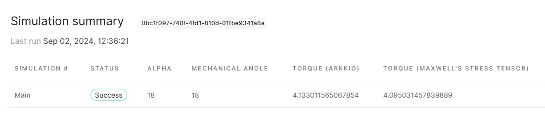

   

References

Footnotes

1. Arkkio’s Method for Torque Computation, https://www.anttilehikoinen.fi/research-work/arkkios-method-torque-computation/ ↩