
SC 002 - Twisted superconductor AC Loss
In this tutorial, AC loss in a high-temperature superconducting (HTS) wire is simulated using the H-φ formulation.
Model definition
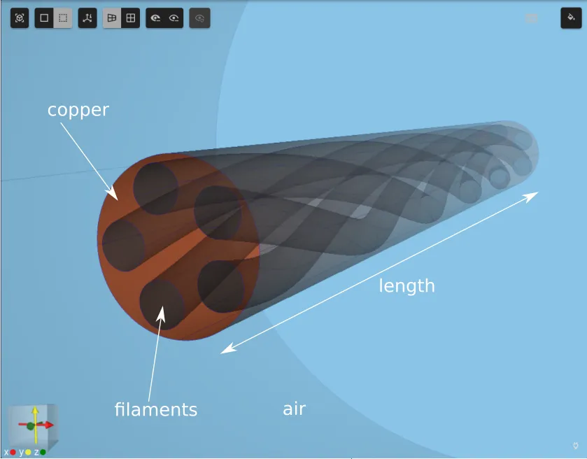
Section titled “Model definition”The wire consists of twisted superconducting filaments embedded into a copper matrix. The whole modelling domain with an air cylinder around the wire is illustrated below.
| Element | Dimension |
|---|---|
| Air cylinder diameter | 10 mm |
| Copper cylinder diameter | 535 μm |
| Filament diameter | 350 μm |
| Domain length | 10 mm |
Output results
Section titled “Output results”- Joule losses as a function of time in the copper and the superconducting filament regions. The losses over the volume of interest can be computed as
Material Data
Section titled “Material Data”Magnetic permeability, :
- all domains:
Electric resistivity, :
- Copper:
- Superconducting filaments:
-
- Critical electric field strength,
- Exponent,
- Critical electric current,
- Total cross-section are of superconducting filaments,
- Critical electric current density,
-
Source
Section titled “Source”The problem is sourced by applying a total current of
where the frequency is .
Step-by-step guide
Section titled “Step-by-step guide”Here you’ll find a detailed step-by-step tutorial on how to simulate AC loss in a twisted filament HTS wire Quanscient Allsolve.
Step 1 - Import the geometry
Section titled “Step 1 - Import the geometry”-
Start with a new project and name it as
SC twisted filament AC loss -
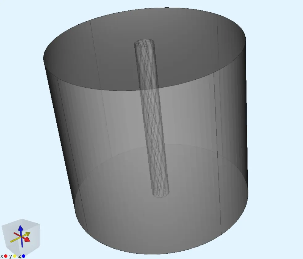
Import the geometry as a
.stepfile with default import options.File download link: twisted-superconductor.step
-
Confirm model changes.
Step 2 - Define regions
Section titled “Step 2 - Define regions”-
Go to the
Commonsidebar. -
Define a region for air:
Region name Region type Target airVolume Air cylinder 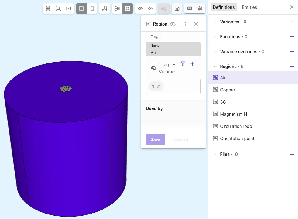
-
Define a region for copper:
Region name Region type Target copperVolume Copper matrix 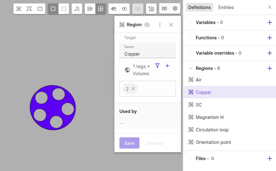
-
Define a region for the superconducting filaments:
Region name Region type Target scVolume SC filaments 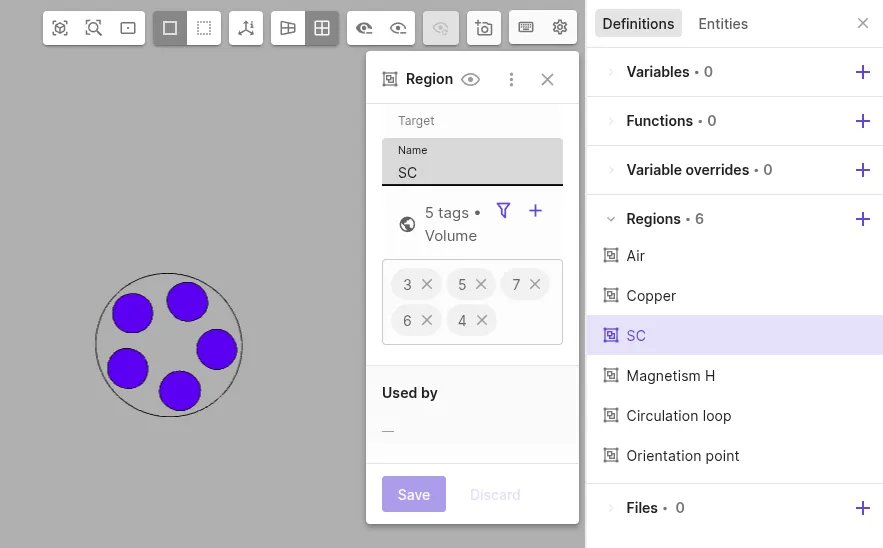
Step 3 - Define materials
Section titled “Step 3 - Define materials”-
Assign the Air material to the
airregion: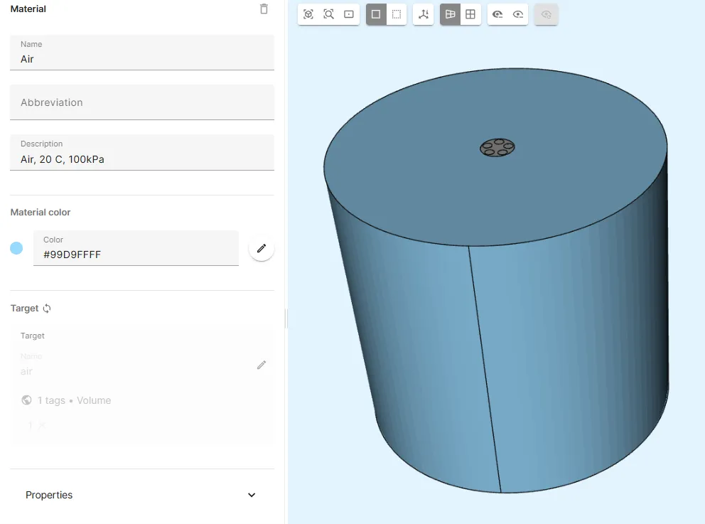
-
Assign the Copper material to the
copperregion: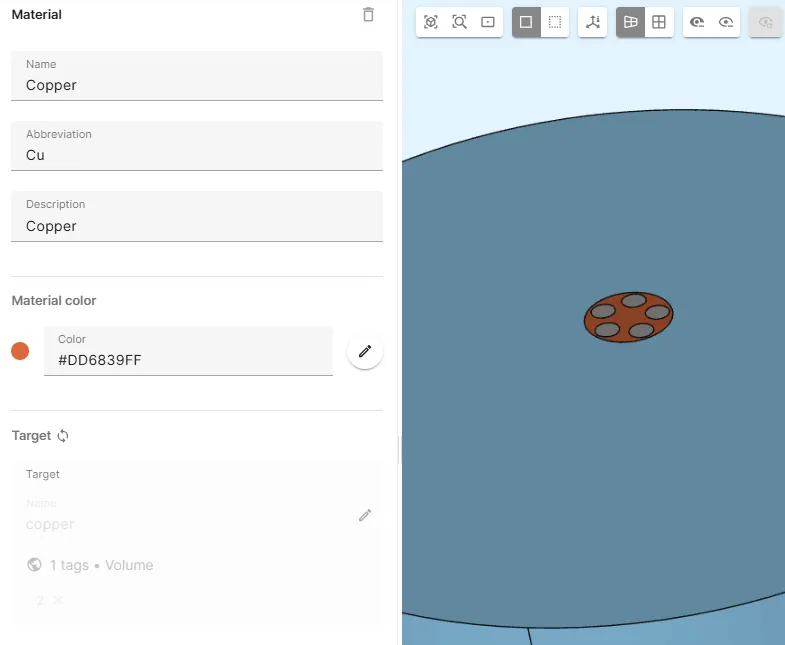
-
Assign the YBCO superconductor material to the
scregion: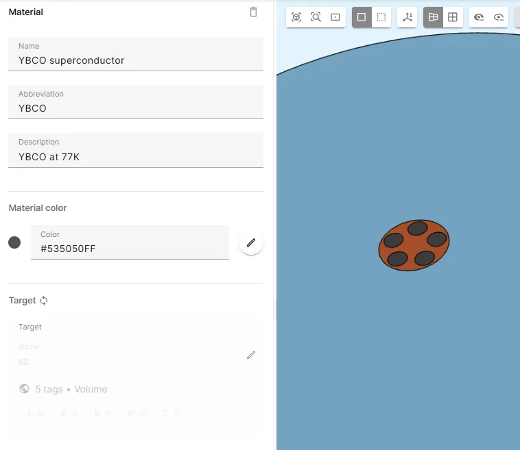
Step 4 - Define variables
Section titled “Step 4 - Define variables”-
Define new variables:
Name Description Expression f Frequency [Hz] 50YBCO_Ic Critical current [A] 100YBCO_Asc Filament cross-section area [m^2] 3.4541e-7Iop Operating current [A] 0.8 * YBCO_Ic * sin(2 * pi * f * t) -
Modify existing variables:
Name Modified expression YBCO_Jc YBCO_Ic / YBCO_AscYBCO_n 30
Step 5 - Define physics and apply the current source
Section titled “Step 5 - Define physics and apply the current source”-
Go to the
Physicssection. -
Add the
Magnetism Hphysics:Physics Target Magnetism H Copper matrix and SC filaments 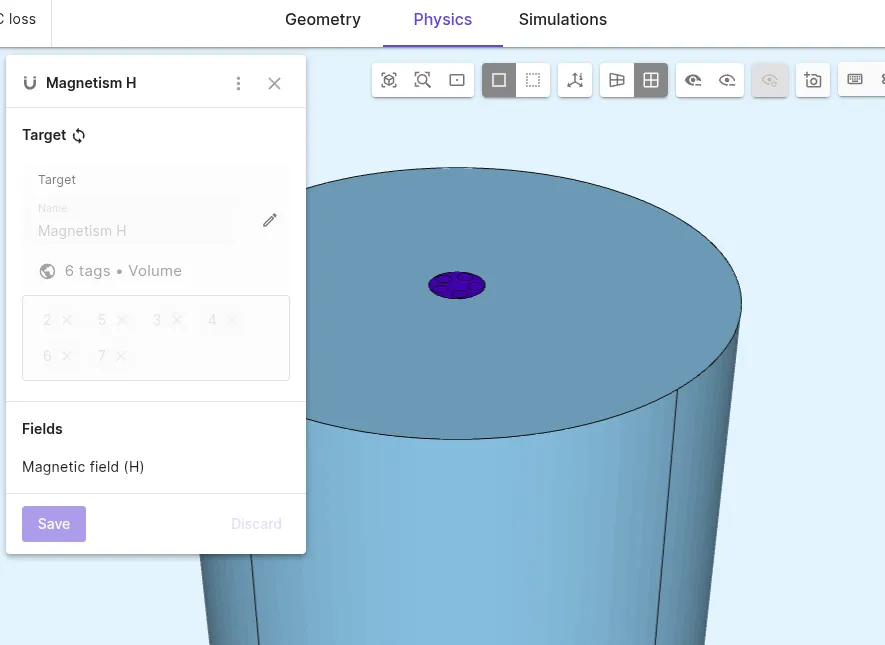
-
Add the
Magnetism φphysics:Physics Target Magnetism φ Air cylinder ( airregion)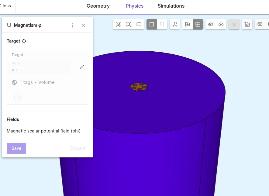
-
Add a
Lump I/V cutinteraction to Magnetism φ.Interaction name Interaction type Target Value Current source Lump I/V cuta counter-clockwise loop at the top edge of the copper matrix Iop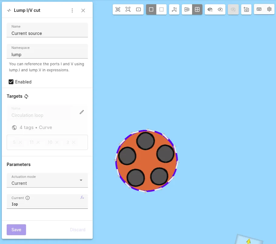
-
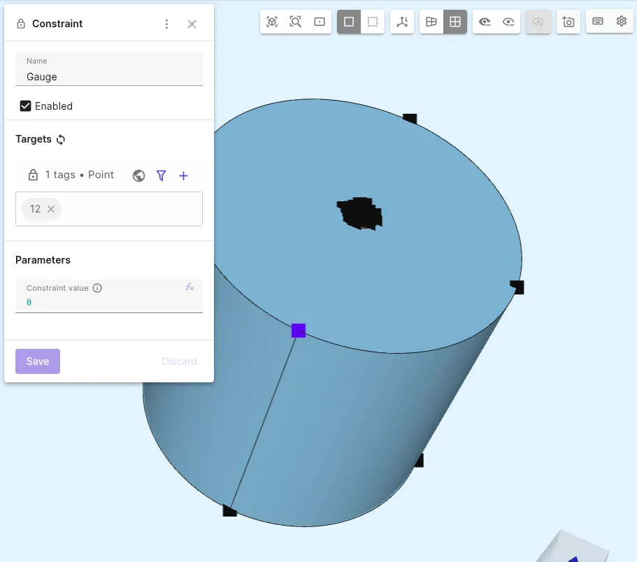
Add a
Constraintinteraction to Magnetism φ:Interaction name Interaction type Target Value Gauge Constrainta point at the external boundary of the air domain 0Any point on the external boundary of the air domain can be selected. This constraint is the gauge condition for the scalar potential φ.
-
Add the
H-φ couplinginteraction to Magnetism H. -
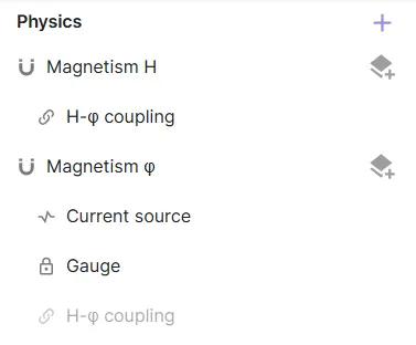
Before moving on, check that your physics tree matches the one below:
Step 6 - Generate a mesh
Section titled “Step 6 - Generate a mesh”-
Go to the
Simulationssection. -
Add a new mesh.
-
Set Autorefine to
Disabled. -
Open the collapsible menu for
Mesh element size. -
Set Curvature enhancement to
25. -
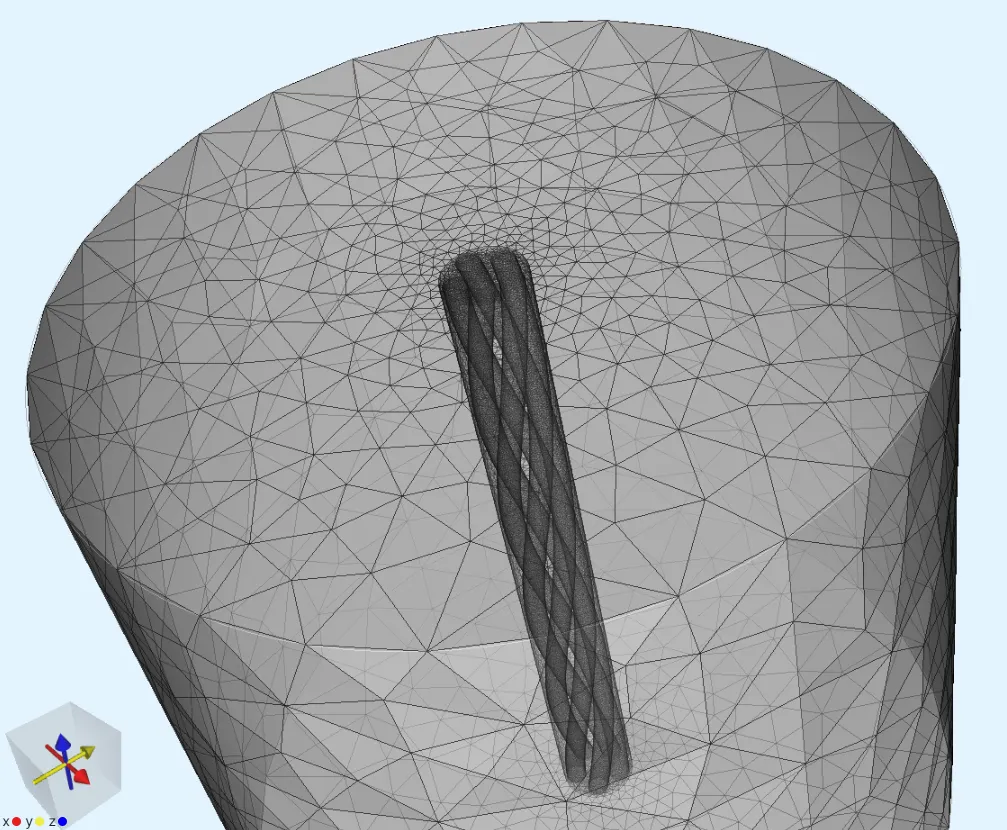
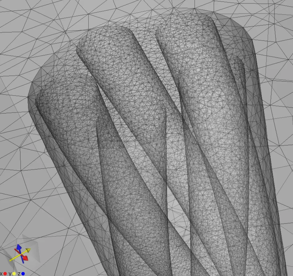
Generate the mesh and check the preview.
Step 7 - Select simulation settings
Section titled “Step 7 - Select simulation settings”-
Add a new simulation.
-
Set Analysis type to
Transient. -
Select Transient settings:
Timestep algorithm Start time [s] End time [s] Timestep size [s] Implicit Euler 00.010.0001 -
Set Solver mode to
Iterative solver. -
Set Node count to
50. -
Select
Mesh 1as the mesh for your simulation. -
Define custom value outputs for computing Joule losses in the filaments and copper:
Output name Output type Output expression SC loss Custom value output integrate(reg.sc, transpose(E) * j, 4)Cu loss Custom value output integrate(reg.copper, transpose(E) * j, 4)In the expressions above,
Eandjare 3 x 1 column vectors.transpose(E)creates a 1 x 3 row vector fromEso that the multiplication withjproduces a dot product . The last argument4is the integration order. -
Open the Script for your simulation.
-
Enable
Scripting mode. -
Replace the first autogenerated line under
# Magnetism Hwith the following Newton-linearization [4]:rho = 1/par.sigma(df.j)dedj = rho*qs.eye(3) + (expr.YBCO_n-1.0)*rho/qs.max(df.j*df.j, 1e-40) * df.j * qs.transpose(df.j)dofe = rho*df.j + dedj * (qs.curl(qs.dof(fld.H))+var.curl_dof_Hs - qs.curl(fld.H)-var.curl_Hs)form += qs.integral(reg.sc, dofe * (qs.curl(qs.tf(fld.H)) - var.curl_tf_Hs))form += qs.integral(reg.copper, qs.inverse(par.sigma(df.j)) * (qs.curl(qs.dof(fld.H)) + var.curl_dof_Hs) * (qs.curl(qs.tf(fld.H)) - var.curl_tf_Hs))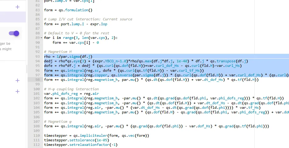
Step 8 - Run the simulation and see results
Section titled “Step 8 - Run the simulation and see results”-
Run the simulation.
-
To follow the simulation progress, open
Logs. -
The SC and Cu loss results can be seen in
Plotting, even while the simulation is running: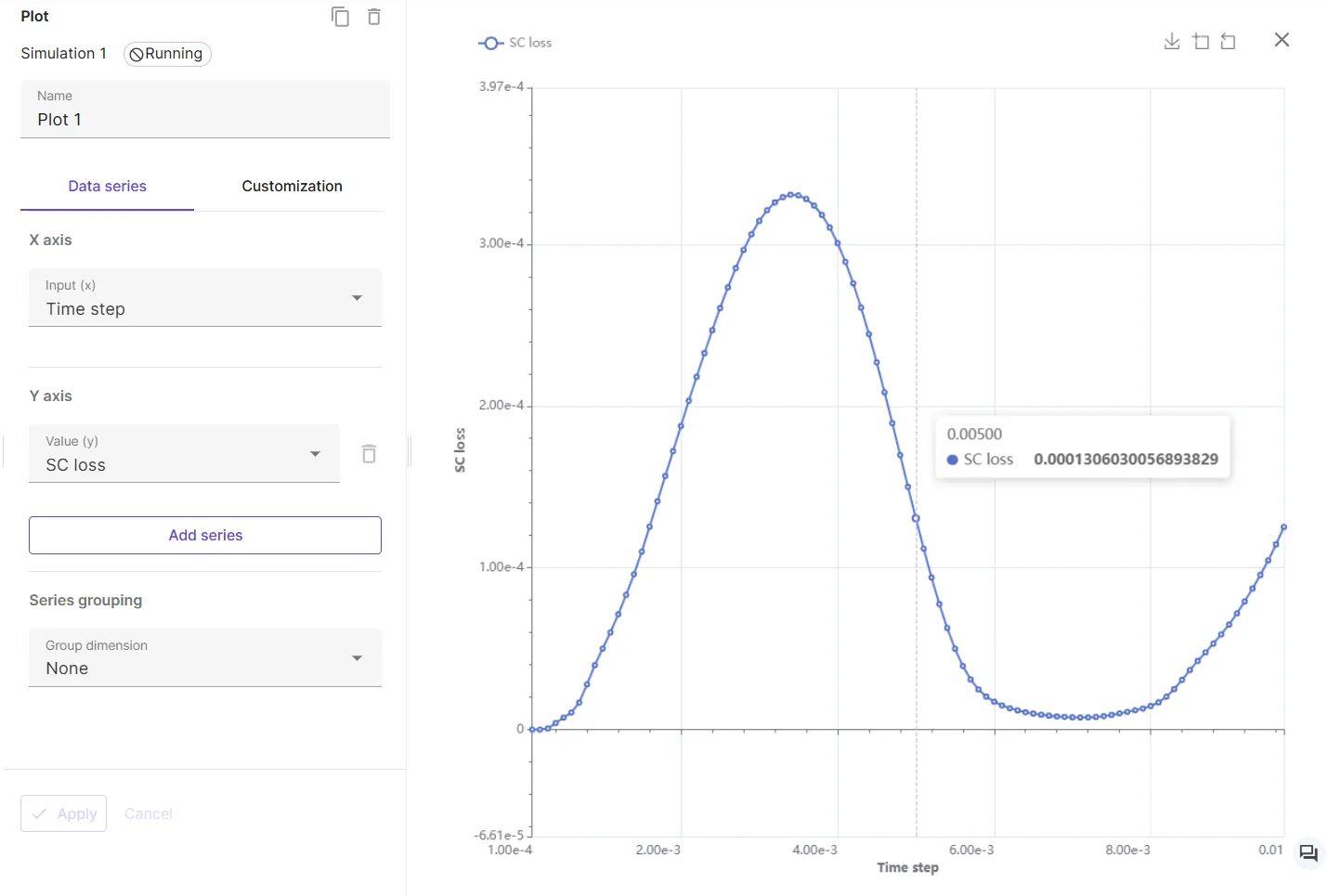
References
Section titled “References”[1] H-φ Formulation in Sparselizard Combined With Domain Decomposition Methods for Modeling Superconducting Tapes, Stacks, and Twisted Wires. https://doi.org/10.1109/TASC.2023.3240389
[2] Allsolve demo project of Superconductor AC losses. https://allsolve.quanscient.com/#/projects/demo/8fed82d1-5bf0-4c02-835b-94e65a60f847
[3] Youtube tutorial of Superconductor AC losses. https://youtu.be/B9QZZ5y7RpQ
[4] Newton Linearization. https://en.wikiversity.org/wiki/Nonlinear_finite_elements/Newton_method_for_finite_elements