SC 001 - HTS tape AC loss

What you’ll learn

• How to import a mesh file, define regions for multi-layered domains, and assign materials (including a custom Hastelloy material).
• How to set up the H-φ formulation with Magnetism H and Magnetism φ physics, apply a Lump I/V cut current source, and define variables and functions for the YBCO power law.
• How to modify the simulation script with Newton-Raphson linearization and run a transient simulation.
• How to plot Joule loss outputs and visualize current density with slice and glyph filters.

In this step-by-step tutorial, AC power loss in a high-temperature superconducting (HTS) tape is simulated.

HTS materials are defined as having a relatively high critical temperature of above 77 K. ¹

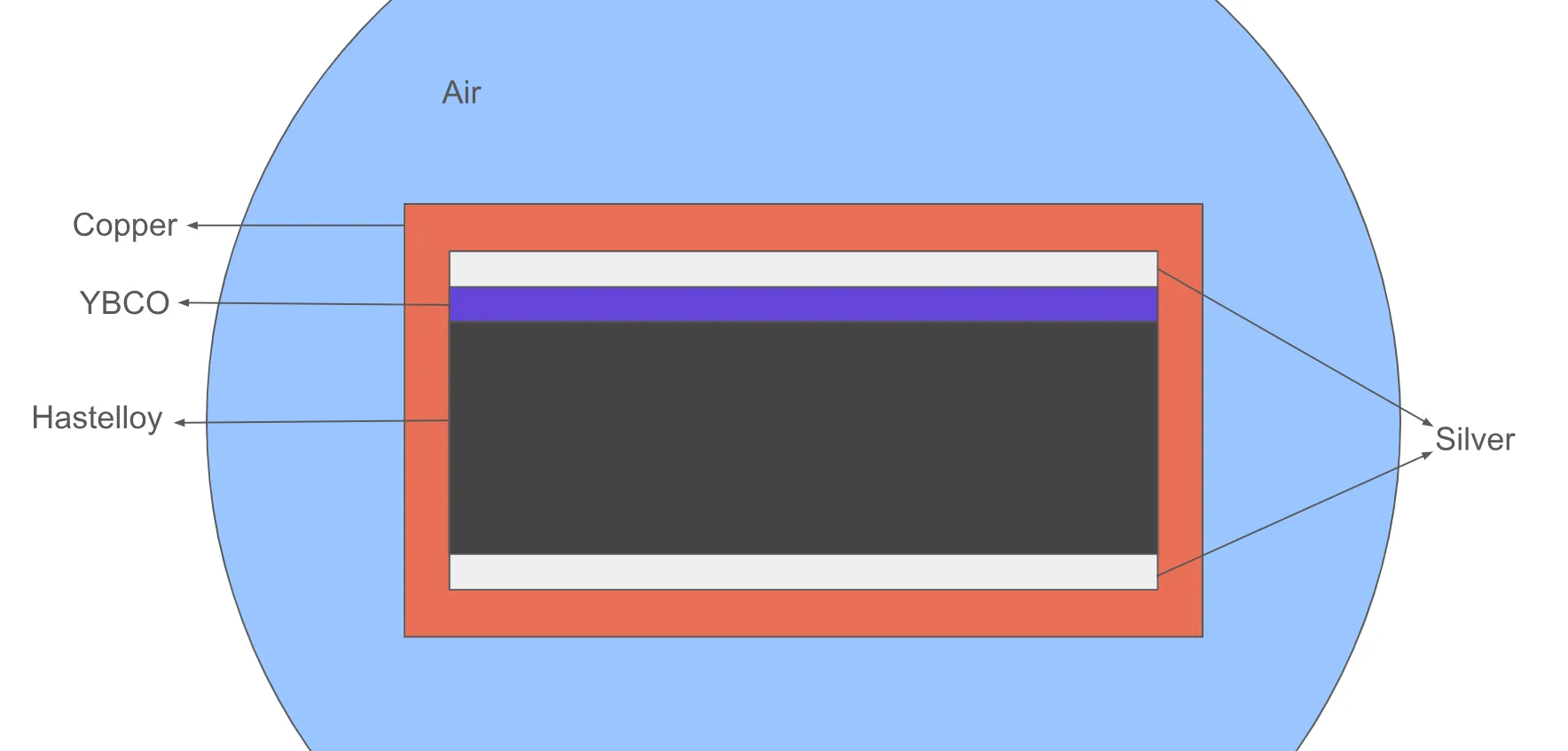
Model definition

The tape model is multi-layered, with the superconducting YBCO (Yttrium barium copper oxide) layer taking up only a small part of the tape cross-section. Hastelloy is used as substrate, which forms the thick middle layer of the tape. Copper is used on the outer layer as a stabilizer.

A reference image of the tape cross-section (not to scale) is depicted below.

Model geometry

Element	Dimensions
air cylinder	radius = 8 cm
tape	width = 4 mm, height = 95 μm, length = 1 cm
copper layer	thickness = 20 μm
silver layer	thickness = 2 μm
YBCO layer	thickness = 1 μm
hastelloy layer	thickness = 50 μm
domain	length = 1 cm
YBCO cross-section	$A_{\rm YBCO}$ = $3.96 \cdot 10^{-9}$ m²

Material Data

Magnetic permeability ($\mu$)

• all domains: $\mu_0$

Electric resistivity ($\rho$)

• Hastelloy: $10^{-6}~\Omega$m
• Silver: $10^{-8}~\Omega$m
• Copper: $10^{-8}~\Omega$m
• YBCO:
  • $\rho=\frac{E_c}{J_c}\left(\frac{||J||}{J_c} \right)^{n-1}$
    • $E_c = 100$ μV/m
    • $n=30.5$
    • $J_c=2.85\times 10^{10}$ [A/m$^2$]
    • $I_c=J_c\cdot A_{\rm YBCO}$
  • $E\approx E^0+\frac{\partial E}{\partial J}(J-J^0)$

Inputs - case 1

• Frequency $f=50$ Hz

• Operation current $I_{\rm op}(t) = 0.8 ~ I_c \cdot \sin (2 \pi f t)$

• External magnetic flux density $B_{\rm ext}(t)=0$ [T]

Inputs - case 2

• Frequency $f=50$ Hz

• Operation current $I_{\rm op}(t)=0$ A

• External magnetic flux density $B_{\rm ext}(t) = 20 \cdot \sin (2 \pi f t)$ [mT]

Output results

• Joule losses in the YBCO region, and in the normalconducting region

$$\begin{equation} P_i(t)=\int_{\Omega_{i}}\boldsymbol{E}(t)\cdot \boldsymbol{J}(t)~\rm{d}\Omega \end{equation}$$

• Field visualizations

Step-by-step guide

Here you’ll find a detailed step-by-step tutorial on how to simulate AC Loss in an HTS tape in Quanscient Allsolve.

Step 1 - Create the project and import geometry

1. Create a new project and name it as HTS tape tutorial, for example.

2. Import the model as a mesh file.

   • File download link: htstape.msh

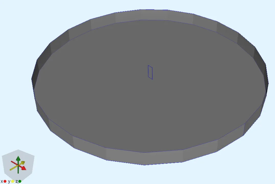
The air cylinder takes up most of the model view, with the smaller tape volume in the middle.

Step 2 - Define regions

1. Open the Common sidebar.

2. Define regions:

   Region name	Region type	Target
   air	Volume	Air cylinder
   copper	Volume	Copper layer
   silver	Volume	Silver layers
   hastelloy	Volume	Hastelloy layer
   ybco	Volume	YBCO layer
   normalconducting	Volume	Silver, hastelloy, and copper layers

Pick with rule

If selecting thin tape layers on the model view is difficult, use the Pick with rule tool to select correct entities for the regions.

Step 3 - Define the materials

1. Go to the Physics section.

2. Assign the Air, Silver, Copper and YBCO materials to their corresponding regions.

   Note: YBCO power law

   When the YBCO material is added, predefined variables and a function related to the YBCO power law are automatically created. See them in the Common sidebar.

3. In Silver and Copper material properties, change Electric conductivity to 1e8.

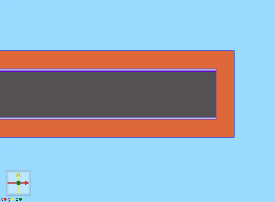
4. Create the new material Hastelloy and add its properties:

   Material name	Color	Target
   Hastelloy	Dark grey	hastelloy region

   Material property	Value
   Electric conductivity	1e6
   Magnetic permeability	mu0

5. (Optional) Change the YBCO material color to purple in order to distinguish it from hastelloy.

Finished materials:

Step 4 - Define variables & functions

Go to the Common sidebar.

1. Edit predefined variables:

   Name	Updated expression
   YBCO_Jc	2.85e10
   YBCO_n	30.5

2. Define new variables:

   Name	Description	Expression
   freq	Frequency [Hz]	50
   Bext	External magnetic flux density [T]	0
   Aybco	YBCO layer cross-section area [m^2]	3.96e-9
   Iop	Operating current [A]	0.8 * YBCO_Jc * Aybco * sin(2 * pi * freq * t)

Step 5 - Define physics and boundary conditions

Go to the Physics section.

Add the Magnetism φ and Magnetism H physics before moving on to set up their interactions.

Physics 1 - Magnetism φ

1. Set the Magnetism φ target:

   Physics	Target
   Magnetism φ	air region

2. Add a constraint interaction to Magnetism φ:

   Interaction name	Interaction type	Target	Value
   Constraint	Constraint	point at the outer edge of the air cylinder	0

3. Add an External field interaction to Magnetism φ:

   Interaction name	Interaction type	Target	Value
   External field	External field	outer surface of the air cylinder	[0; Bext; 0]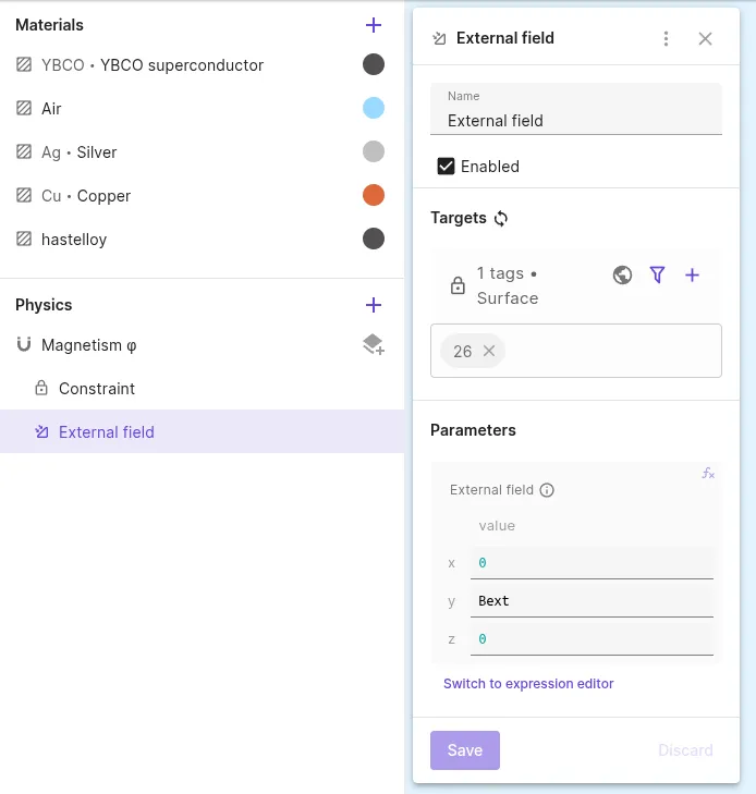

   

4. Add a Lump I/V cut interaction to Magnetism φ:

   Interaction name	Interaction type	Target	Actuation mode	Current
   Lump I/V cut	Lump I/V cut	a loop around the tape cross-section	Current	Iop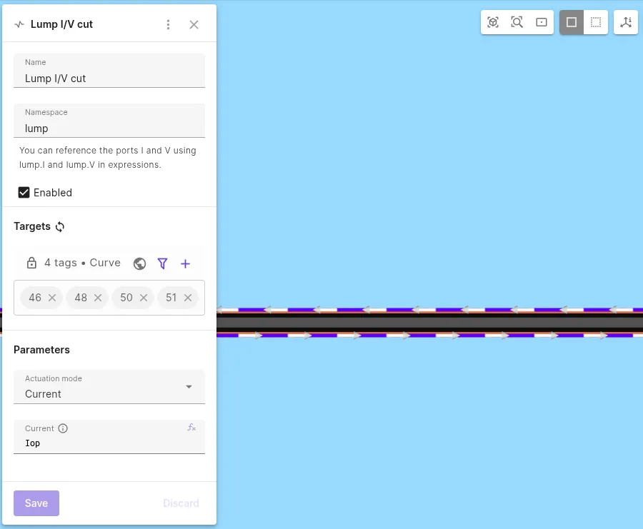

   

Physics 2 - Magnetism H

1. Set the Magnetism H target:

   Physics	Target
   Magnetism H	All tape-layer volumes. The air cylinder is excluded

2. Add H-φ coupling to Magnetism H.

Step 6 - Select simulation options

1. Go to the Simulations section.

2. Add a new simulation.

3. Set Analysis Type to Transient.

4. Select timestepping options:

   Timestep algorithm	Start time [s]	End time [s]	Timestep size [s]
   Implicit Euler	0	1/freq	1/freq/50

5. Select the imported mesh as the mesh for your simulation.

Step 7 - Add simulation outputs

1. Add custom value outputs for joule loss integrals:

   Name	Output expression
   YBCO loss	integrate(reg.ybco, transpose(E)*j, 4)
   Normalconducting loss	integrate(reg.normalconducting, transpose(E)*j, 4)

2. Add a custom value output for net current:

   Name	Output expression
   Itot	lump.I

3. Add the current density j field output.

4. Toggle Skin only on the j field output.

Step 8 - Modify the simulation script & run

1. Open the simulation Script.

2. Enable Scripting mode.

3. Replace the first line of the autogenerated magnetism H formulation with the following Newton-Raphson linearization:

   rho = 1 / par.sigma(df.j)
   dedj = rho * qs.eye(3) + (expr.YBCO_n - 1.0) * rho / qs.max(df.j * df.j, 1e-40) * df.j * qs.transpose(df.j)
   dofe = rho * df.j + dedj * (qs.curl(qs.dof(fld.H)) + var.curl_dof_Hs - qs.curl(fld.H) - var.curl_Hs)
   form += qs.integral(reg.ybco, dofe * (qs.curl(qs.tf(fld.H)) - var.curl_tf_Hs))
   form += qs.integral(reg.normalconducting, qs.inverse(par.sigma(df.j)) * (qs.curl(qs.dof(fld.H)) + var.curl_dof_Hs) * (qs.curl(qs.tf(fld.H)) - var.curl_tf_Hs))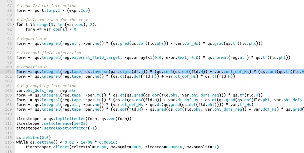

   

   Linearization

   The Newton-Raphson linearization helps in speeding up convergence of nonlinear systems, leading to faster runtimes. In some cases, the nonlinear system does not converge at all with fixed point iteration unless linearized.

4. Save the script.

5. Run the simulation.

Step 9 - Plot & visualize results

Add plots for value outputs and visualizations for field outputs. After adding visualizations and filters, press Render to display the results in the model view.

• The YBCO loss forms two distinct peaks: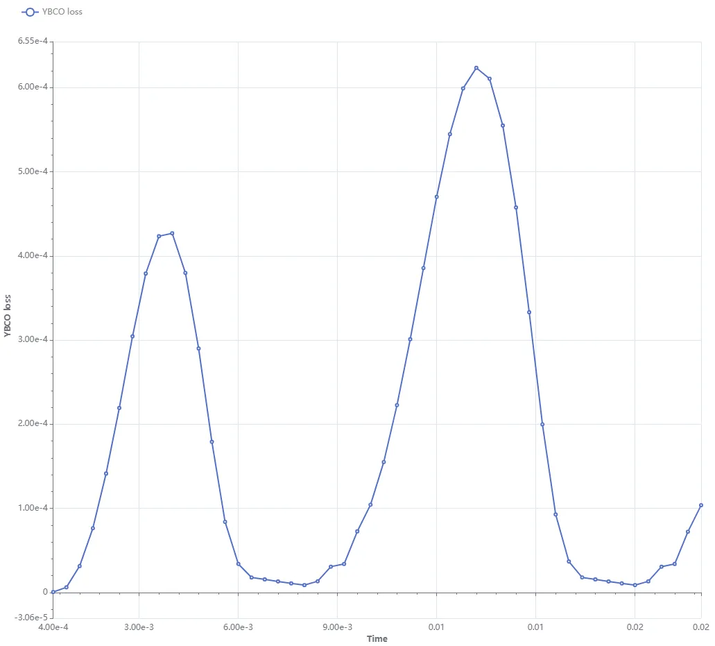

  

• The Normalconducting loss has a similar shape but at a much smaller scale (see Y axis):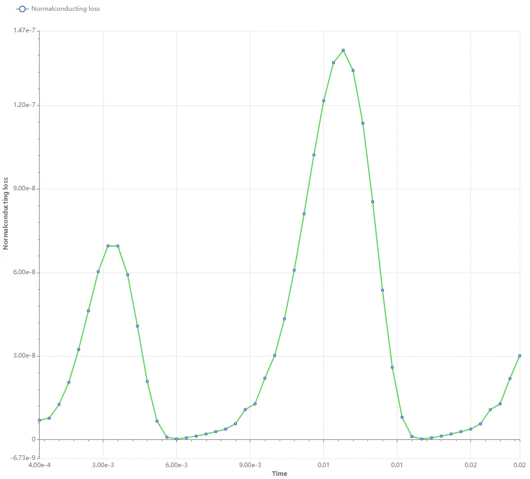

  

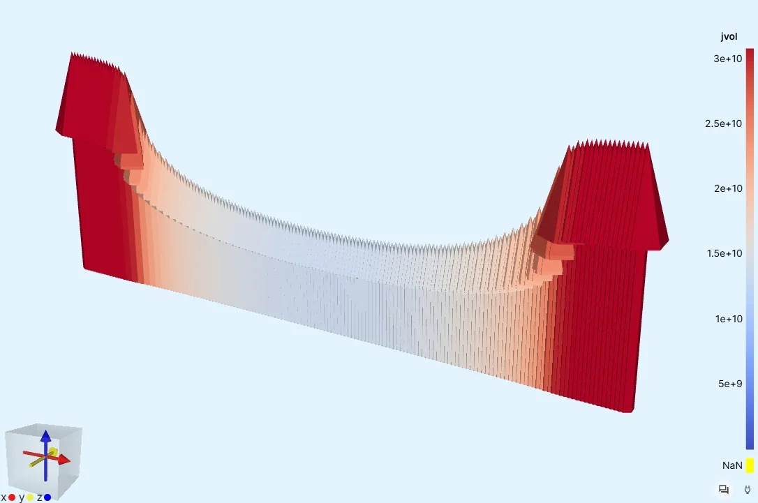
Plotting during simulation

To plot value outputs in real time, add a plot at the start of your simulation.

• To visualize the j field, take a slice at the tape and air cylinder mid-section: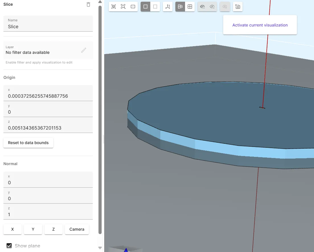

  

• Add a glyph filter on the same visualization. Check the Summary to choose a suitable timestep to visualize. Timestep 33/66 was rendered here:

  

Glyph settings

• If there are too few glyph arrows, increase Max sample points.
• If glyph arrows are too large, decrease Scale factor.

References

Footnotes

1. https://en.wikipedia.org/wiki/High-temperature_superconductivity ↩