
MEMS 003 - Viscoelasticity benchmark
Prerequisites: complete any one step-by-step tutorial first so you are comfortable with the Allsolve project layout (Geometry, Physics, Simulations, Results).
In this MEMS example case, vertical strain is simulated for a rectangular viscoelastic rod. The simulated vertical strain is compared against analytical results.
The model consists of a single box.
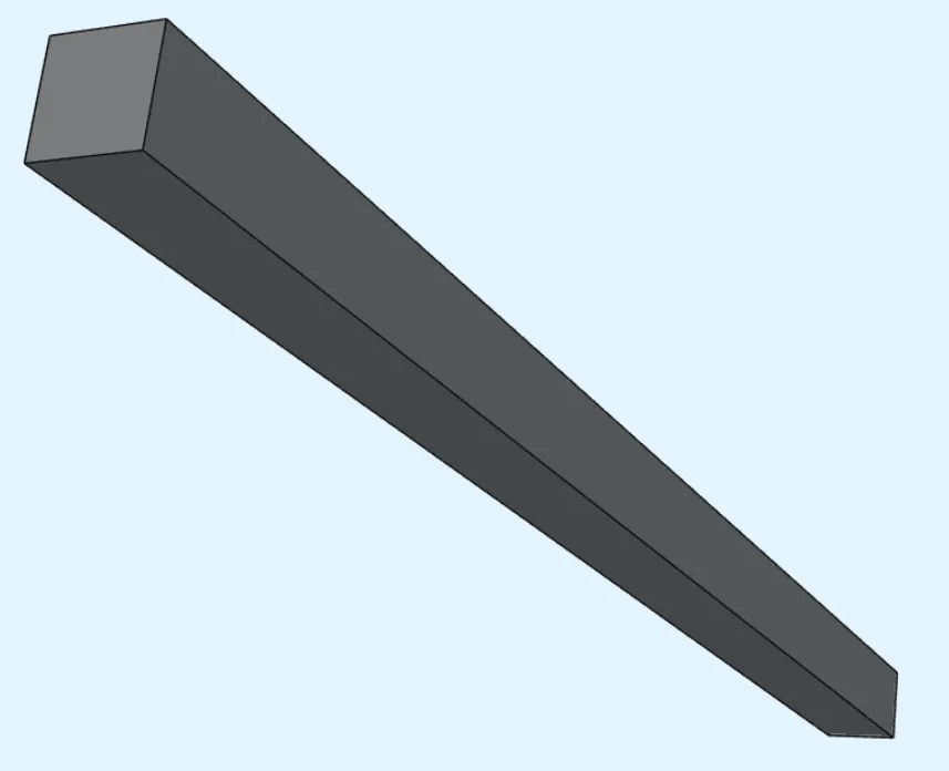
Simulation setup guide
Section titled “Simulation setup guide”Here you’ll find a simplified, example case level guide for setting up a transient viscoelasticity simulation in Quanscient Allsolve.
Step 1 - Define variables
Section titled “Step 1 - Define variables”Create a new project.
Select Box as a starting point and leave model editing for now.
Go to the Common sidebar and define variables:
| Name | Description | Expression |
|---|---|---|
| L | Rod length [m] | 0.002 |
| E0 | Long-term Young’s modulus [N/m^2] | 70e9 |
| E1 | Prony Young’s modulus [N/m^2] | 20e9 |
| tau | Relaxation time [s] | 5e-2 |
Step 2 - Set rod dimensions
Section titled “Step 2 - Set rod dimensions”Now back in the Geometry section, edit dimensions of your Box:
| Name | Element type | Center point [m] | Size [m] | Rotation [deg] |
|---|---|---|---|---|
| box | Box | X: 0 |
X: L/20 |
X: 0 |
Y: 0 |
Y: L/20 |
Y: 0 |
||
Z: 0 |
Z: L |
Z: 0 |
Apply the new dimensions and build.
The box is now tiny, so use Reset view in model view controls to zoom it back into view.
Confirm model changes before moving on.
Step 3 - Define the material
Section titled “Step 3 - Define the material”In the Physics section, define a new material:
| Name | Abbreviation | Target |
|---|---|---|
Benchmark material |
bm |
The box volume |
- Add the material target as a region.
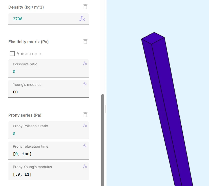
Add material properties:
| Density | Elasticity matrix | Prony series |
|---|---|---|
2700 |
Poisson’s ratio: 0 |
Prony Poisson’s ratio: 0 |
Young’s modulus: E0 |
Prony relaxation time: [0, tau] |
|
Prony Young’s modulus: [E0, E1] |
Step 4 - Define the physics
Section titled “Step 4 - Define the physics”Go to the Physics section.
Add the Elastic waves physics and let it’s target default to the whole geometry.
Define Elastic waves interactions:
- Add
Viscoelastic material model.- Select the box volume as target.
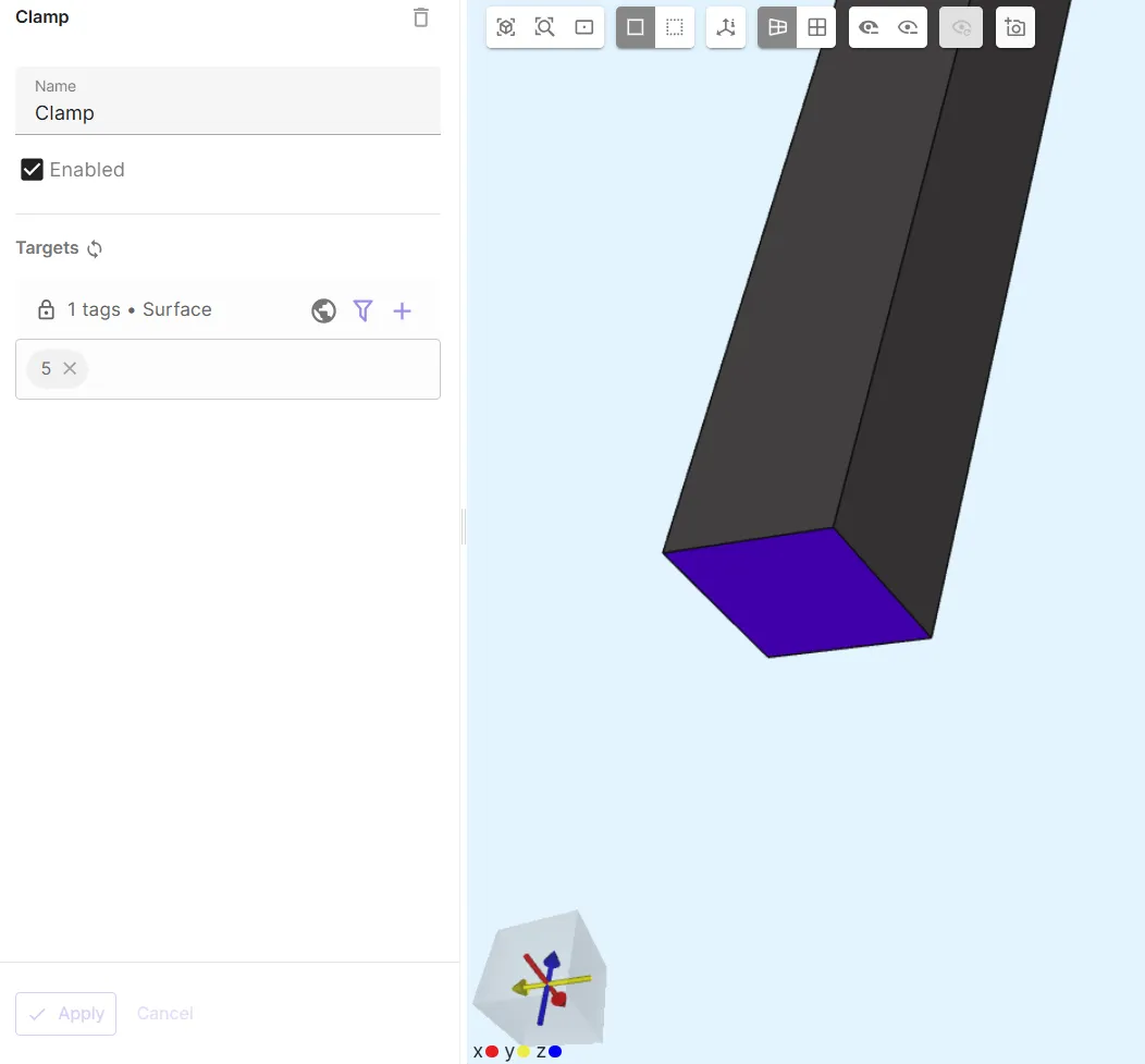
- Add
Clamp.- Select the Z-direction bottom surface as target.
- Add
Load.- As Target, select the Z-direction top surface.
- As Force, input the value
[0; 0; E0]. 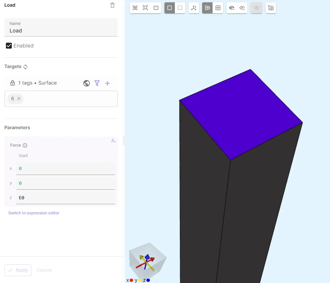
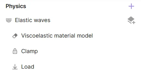
Before moving on, check that your physics tree looks like in the image below.
Step 5 - Generate the mesh
Section titled “Step 5 - Generate the mesh”Go to the Simulations section and create a new mesh:
- Under
Customizations, addTransfinite meshingtargeting the box volume.- Set Segment counts to
25for the long side and3for the short sides. 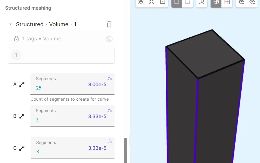
- Set Segment counts to
- Apply settings and mesh.
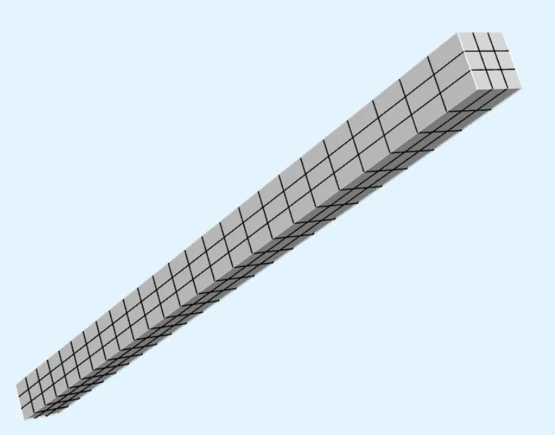
- Check the preview:
Step 6 - Simulate
Section titled “Step 6 - Simulate”In the Simulations section, create a new simulation:
- Set Analysis type to
Transient.- Set Timestep algorithm to
Generalized alpha. - Set Start time (seconds) to
0. - Set End time (seconds) to
0.5. - Set Timestep size (seconds) to
0.0005.
- Set Timestep algorithm to
- As Mesh, select the mesh you made earlier.
- Add Outputs:
- Simulated vertical strain custom value output:
- Name:
Ezz [%] - Output expression:
integrate(reg.benchmark_material_target, compz(grad(compz(u))), 5) / integrate(reg.benchmark_material_target, 1.0, 5)*100
- Name:
- Analytical vertical strain custom value output:
- Name:
Analytical Ezz [%] - Output expression:
100*(1 - E1/(E0 + E1)*exp(-t * E0/tau/(E0 + E1)))
- Name:
- Simulated vertical strain custom value output:
Your simulation is ready to run.
Step 7 - Plot results
Section titled “Step 7 - Plot results”In the Simulations section, add plots to see value output results.
To compare the Ezz [%] and Analytical Ezz [%] results:
- Create a new plot.
- Add both
Ezz [%]andAnalytical Ezz [%]as series on the Y axis. - Customize Y axis Min and Max to
77and101, respectively.
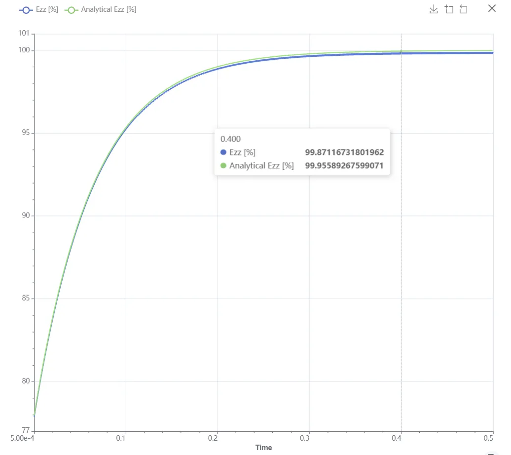
The expected error compared to the analytical result is .
At , Ezz [%] error compared to Analytical Ezz [%] is about .