Loudspeaker in a cabinet

What you’ll learn

• How to set up a multiphysics loudspeaker model coupling Solid mechanics, Current flow, Magnetism A, and Acoustic waves with an air bubble perfectly matched layer (PML).
• How to import CAD files, create custom materials, and define acoustic-structure and A-v couplings.
• How to run a multiharmonic simulation with a frequency sweep and visualize acoustic pressure results.

Prerequisites: work through Bending of a cantilever beam first so you are comfortable with the Allsolve project layout (Geometry, Physics, Simulations, Results).

In this example case, a loudspeaker in a cabinet is simulated.

Loudspeakers are ubiquitous in today’s world. From the compact earbuds that accompany our daily commute to the massive concert sound systems that fill stadiums with music, loudspeakers are essential for delivering audio in various applications.

Simulating sound waves emanating from speaker systems is critical for several reasons. It provides engineers with a valuable tool to:

• Optimize Sound Quality: By understanding how sound waves interact with the speaker’s enclosure and the surrounding environment, engineers can design loudspeaker cabinets that minimize unwanted resonances and distortions, resulting in a cleaner and more accurate sound reproduction.
• Predict Performance: Simulations allow engineers to predict how a loudspeaker will perform in various acoustic settings before physically building the system. This helps identify potential issues and optimize the loudspeaker’s design for its intended use.
• Evaluate New Technologies: Simulations enable engineers to evaluate new materials, speaker designs, and enclosure configurations without the need for expensive and time-consuming prototyping. This accelerates the development of innovative loudspeaker technologies.
• Reduce Development Costs: By minimizing the need for physical prototypes and testing, simulations help reduce development costs and time-to-market for new loudspeaker products.

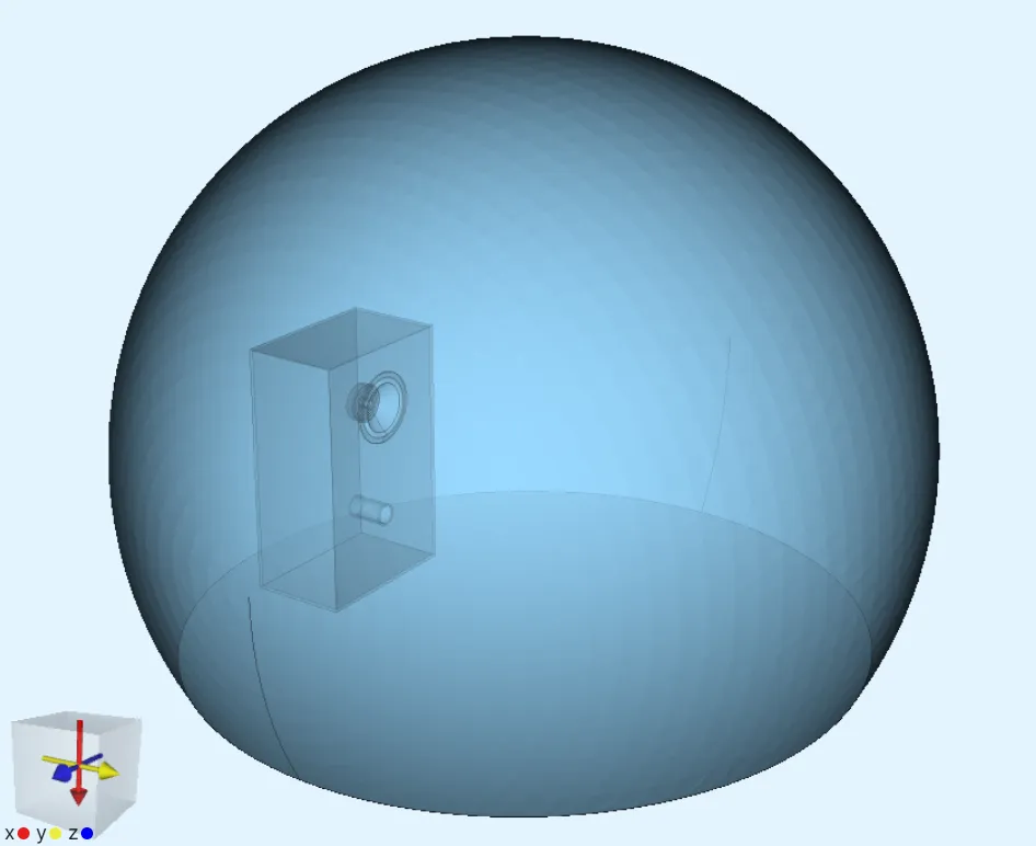
The loudspeaker model used in this example is built in a cabinet, surrounded by an air bubble with a radius of 1 m.

Demo project: LoudspeakerWithCabinet

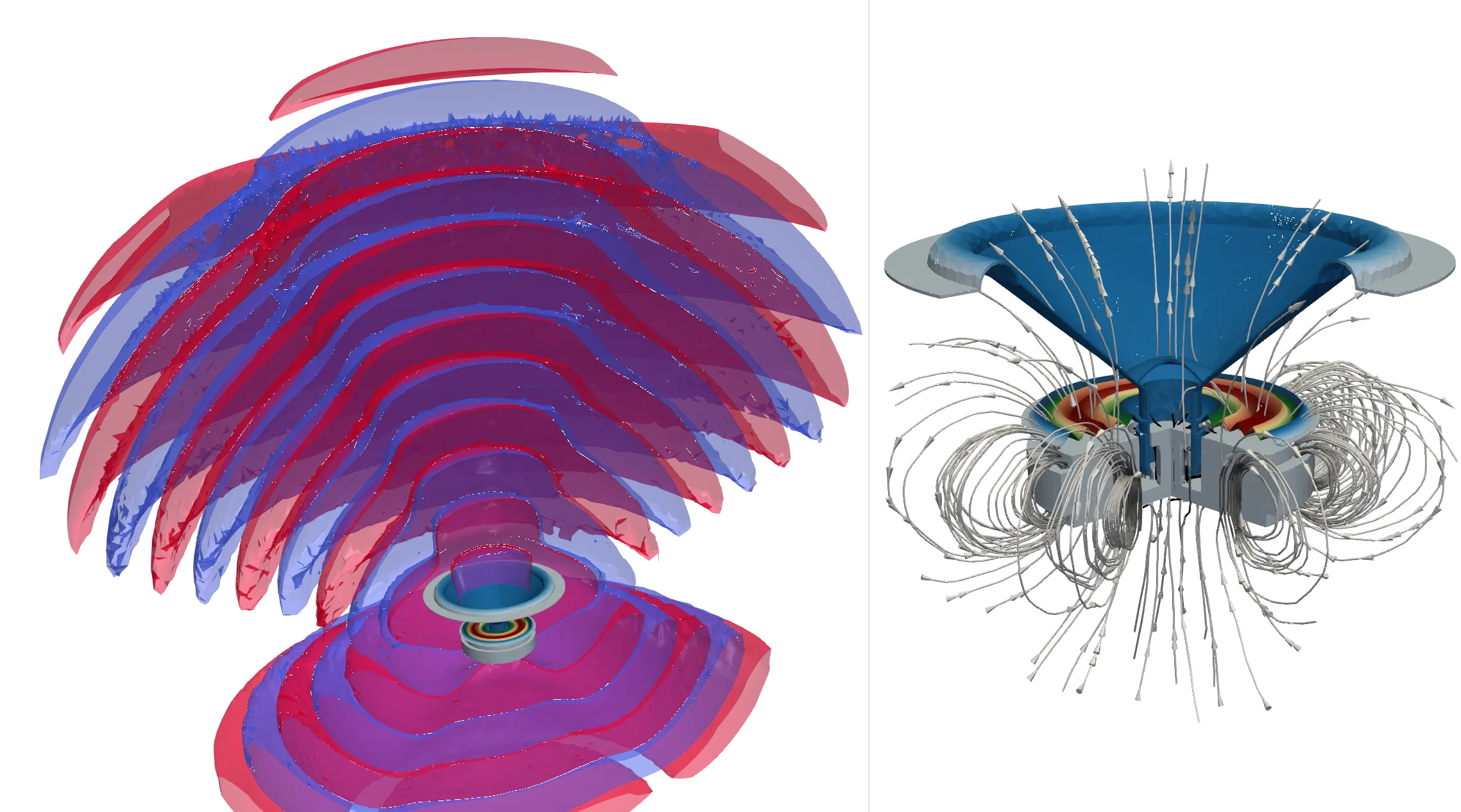
The results of this example were also covered in a Quanscient webinar by Dr. Deshmukh ¹.

Simulation setup guide

Here you’ll find a simplified, example case level guide for setting up a loudspeaker simulation.

Step 1 - Build the geometry

1. In the Geometry section, start off by importing CAD files for your loudspeaker and cabinet.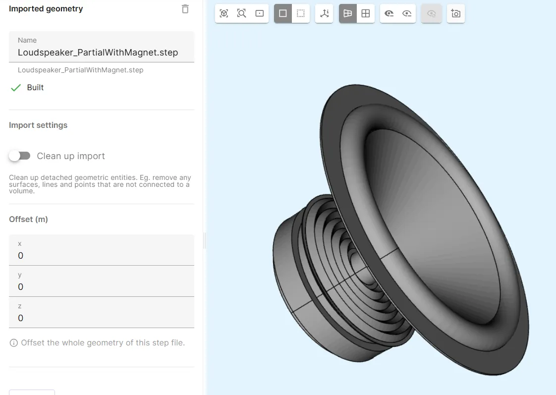

   

   

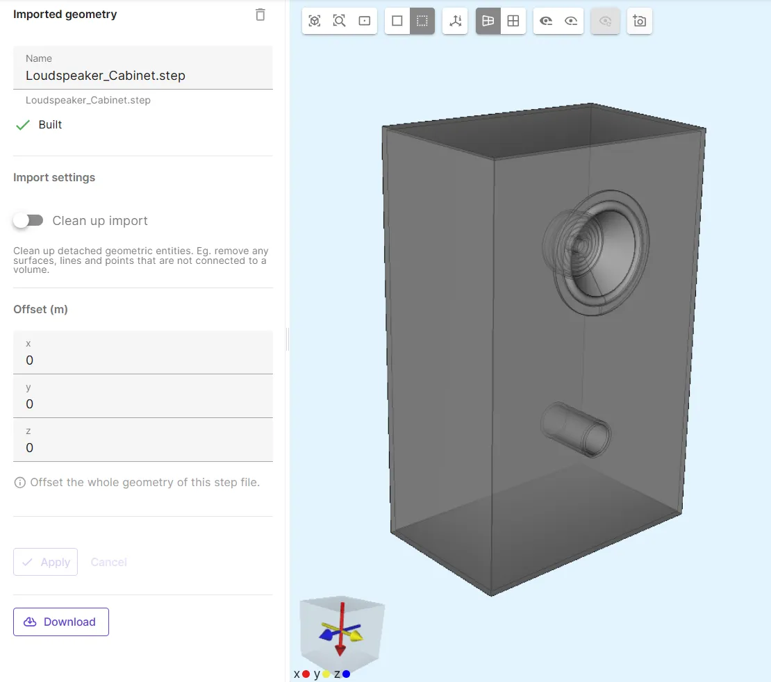
   To try out the .step files used in this example, download them here:

   • Loudspeaker
   • Cabinet

2. Build a sphere for the air bubble geometry:

   Name	Element type	Center point (m)	Radius (m)
   sphere	Sphere	X: 0	1
   		Y: 0.5
   		Z: 0

3. Build a box to cut the sphere in the correct YZ-plane:

   Name	Element type	Center point (m)	Size (m)	Rotation (deg)
   box	Box	X: 0.9975	X: 1	X: 0
   		Y: 0	Y: 4	Y: 0
   		Z: 0	Z: 4	Z: 0

4. Apply the fragment all operation.

5. Apply the remove operation. As target, select the box, the air bubble segment hanging below the loudspeaker, and the thin sliver of loudspeaker cabinet that was cut off by the box.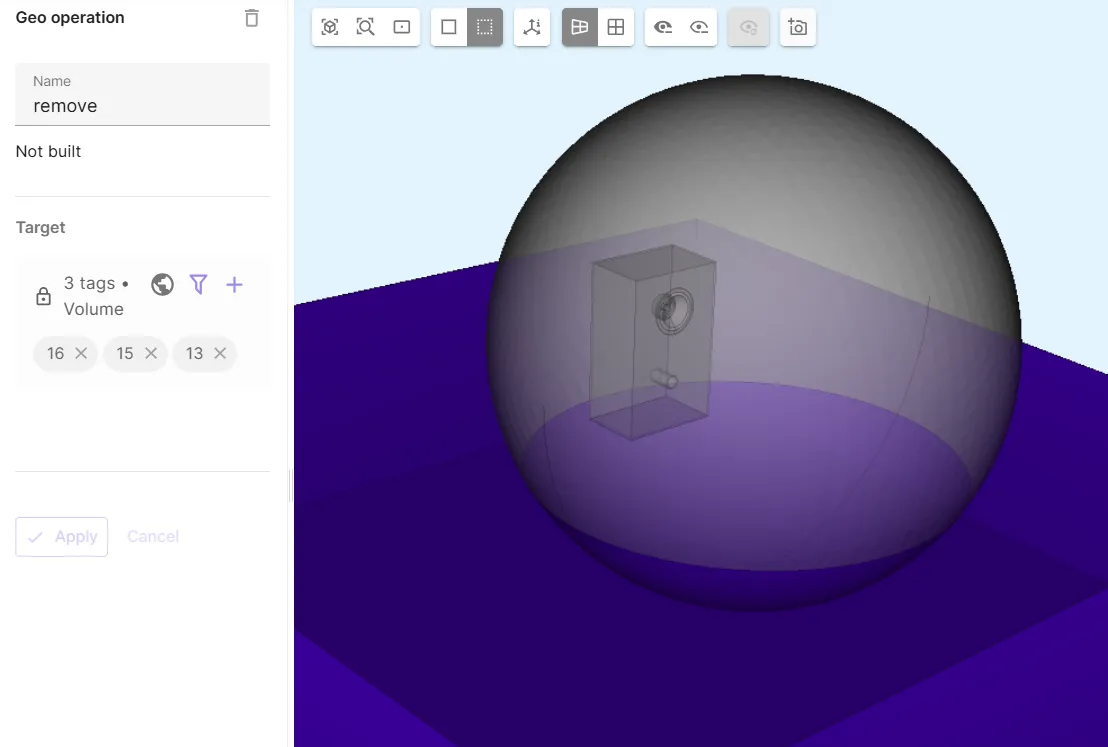

   The air bubble and cabinet bottom surfaces should be level:

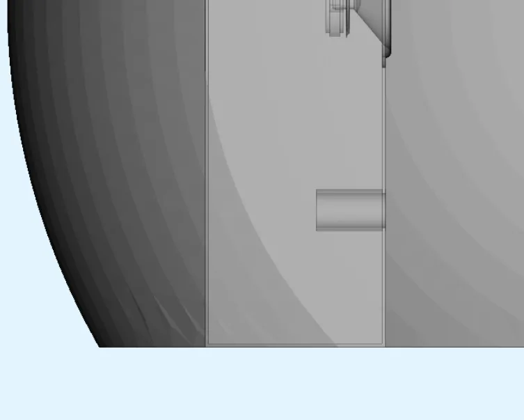
The model geometry is now finished. Confirm model changes before moving on.

Step 2 - Define variables and materials

Proceed to the Common sidebar.

1. Define the following variables:

   Name	Description	Expression
   freq	Frequency (Hz)	3e3

2. Go to the Physics section.

3. Define the model materials:

Material 1 - Air

Assign the Air material to the air bubble volume. Hide the air bubble.

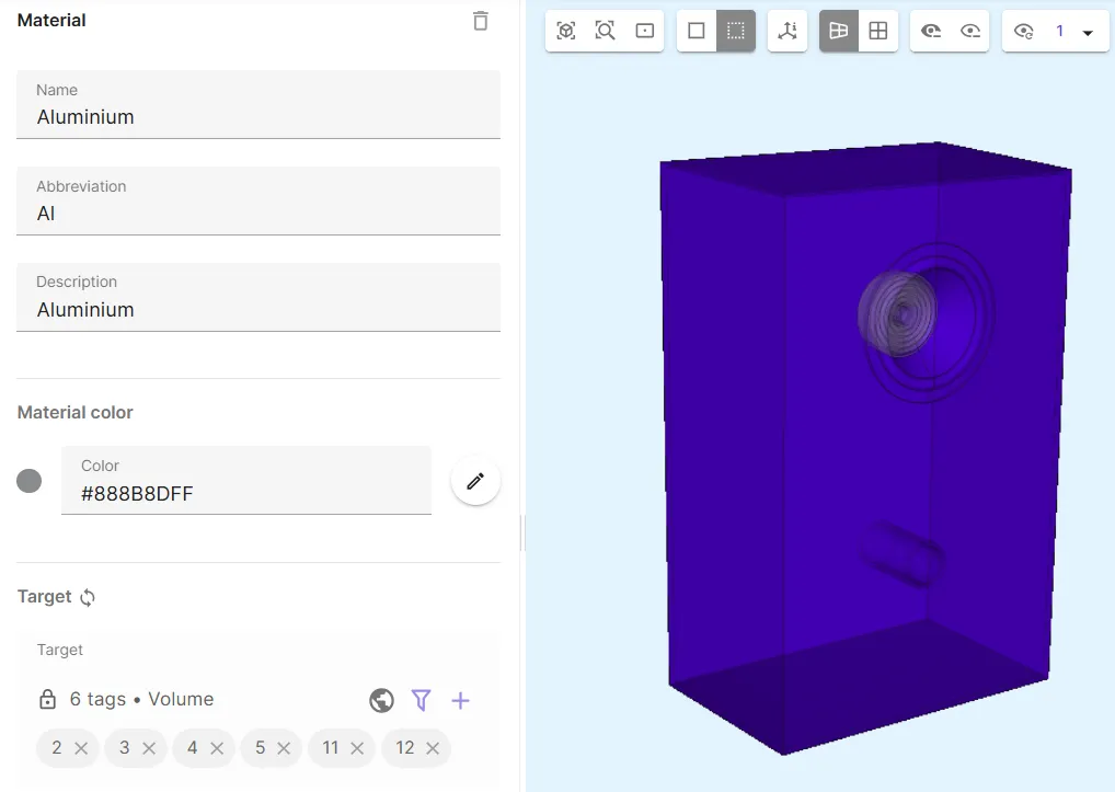
Material 2 - Aluminium

Assign the Aluminium material to the outer cabinet volumes.

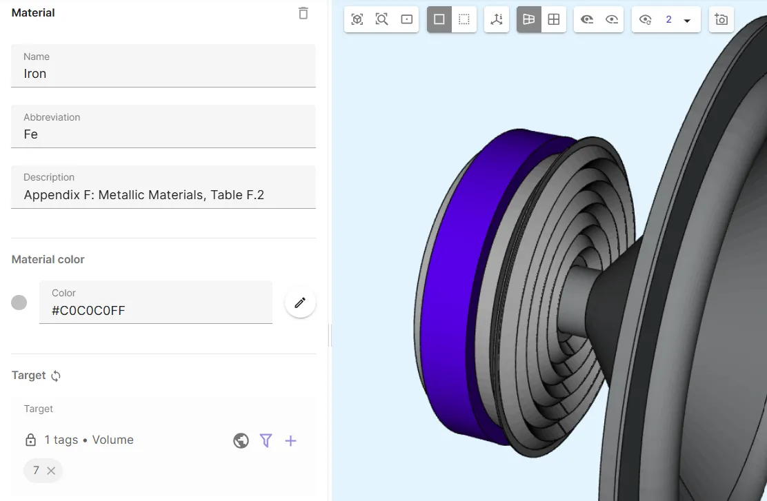
Material 3 - Iron

Assign the Iron material to the magnet volume in the speaker driver.

Edit the iron material properties:

• Change Magnetic permeability to mu0.
• Add Speed of sound with value 5120.

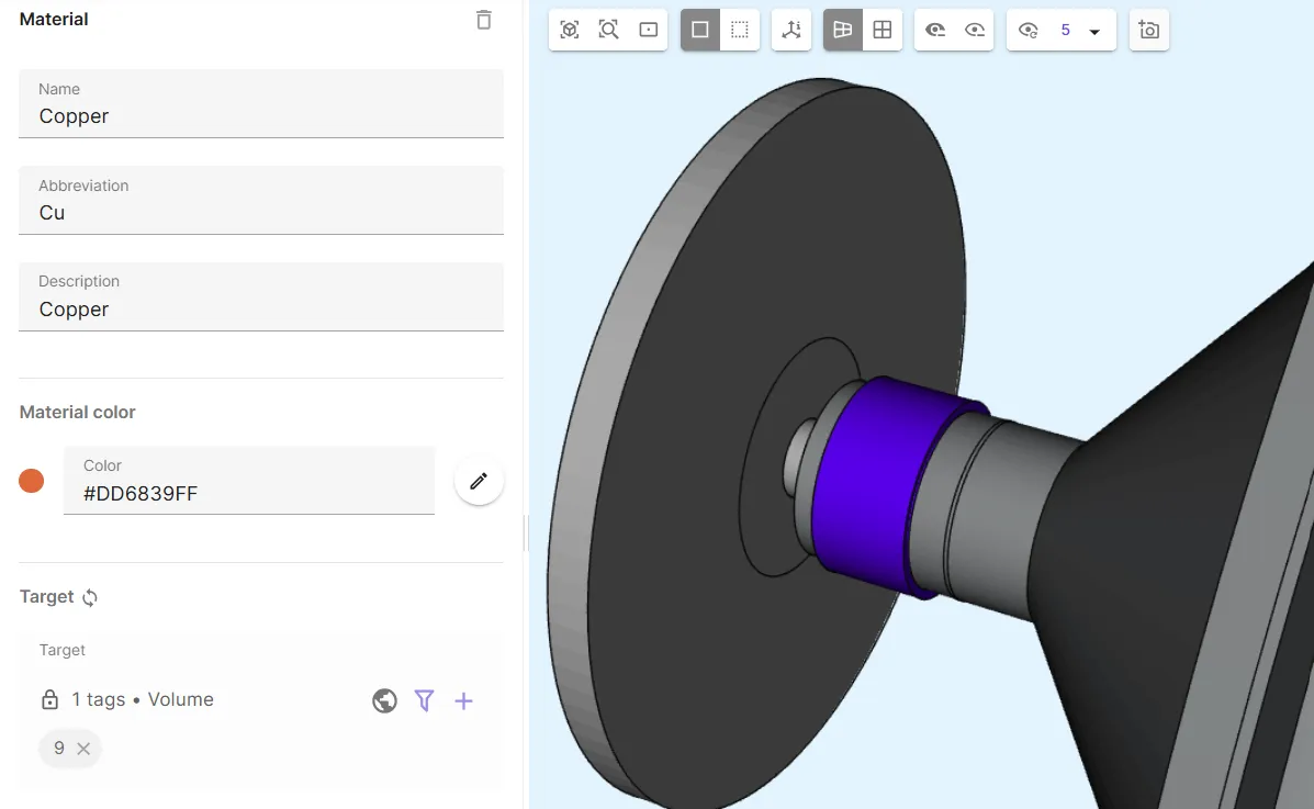
Material 4 - Copper

Assign the Copper material to the homogenized coil volume in the speaker driver.

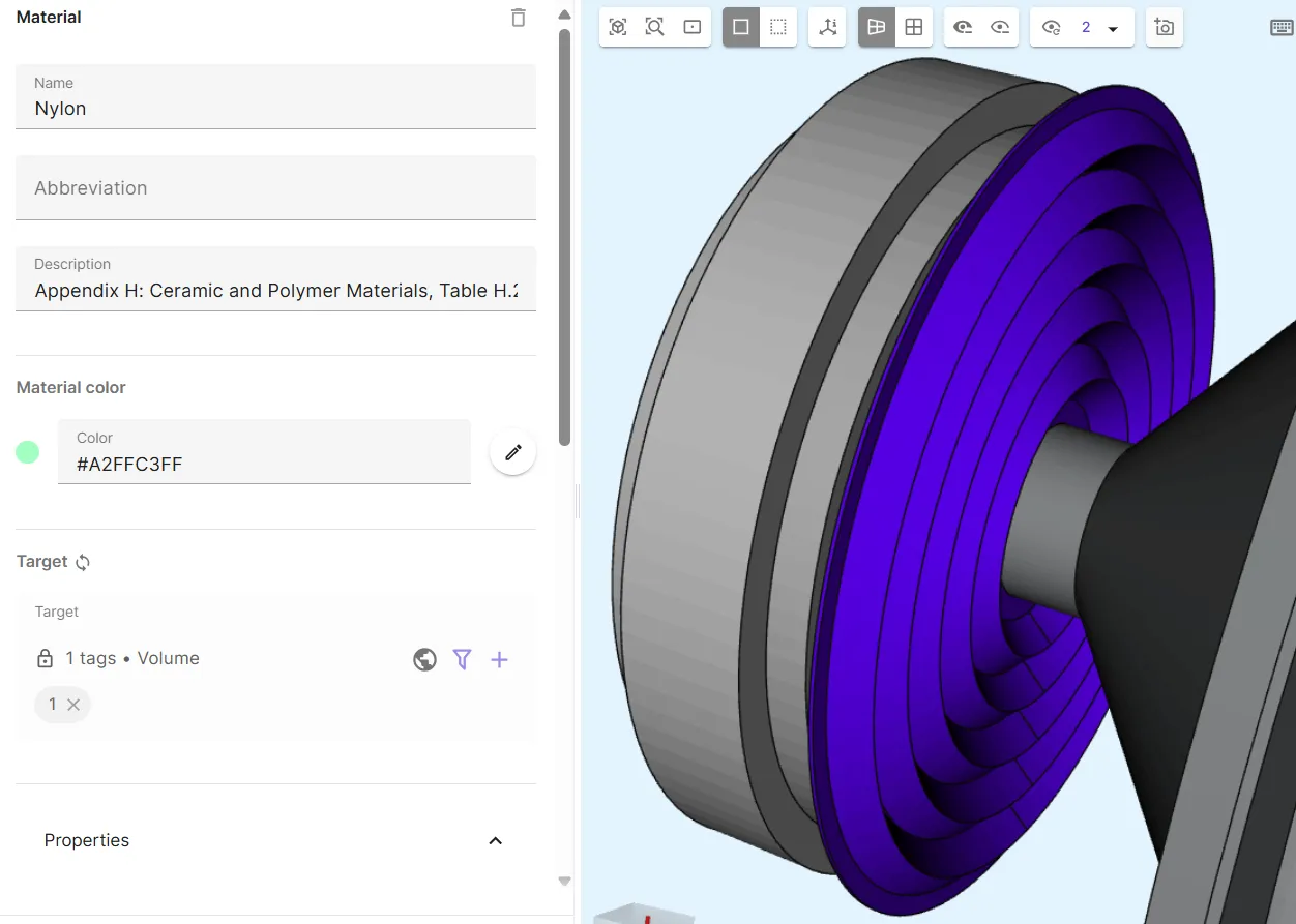
Material 5 - Nylon

Create a new material, Nylon:

• Description
  • Appendix H: Ceramic and Polymer Materials, Table H.2
• Color
  • Turquoise
• Material properties
  • Density: 1150
  • Elasticity matrix:
    • Poisson’s ratio: 0.4
    • Young’s modulus: 3.5e9
  • Electric permittivity: 4.5*epsilon0
  • Magnetic permeability: mu0

Assign your finished Nylon material to the speaker spider volume.

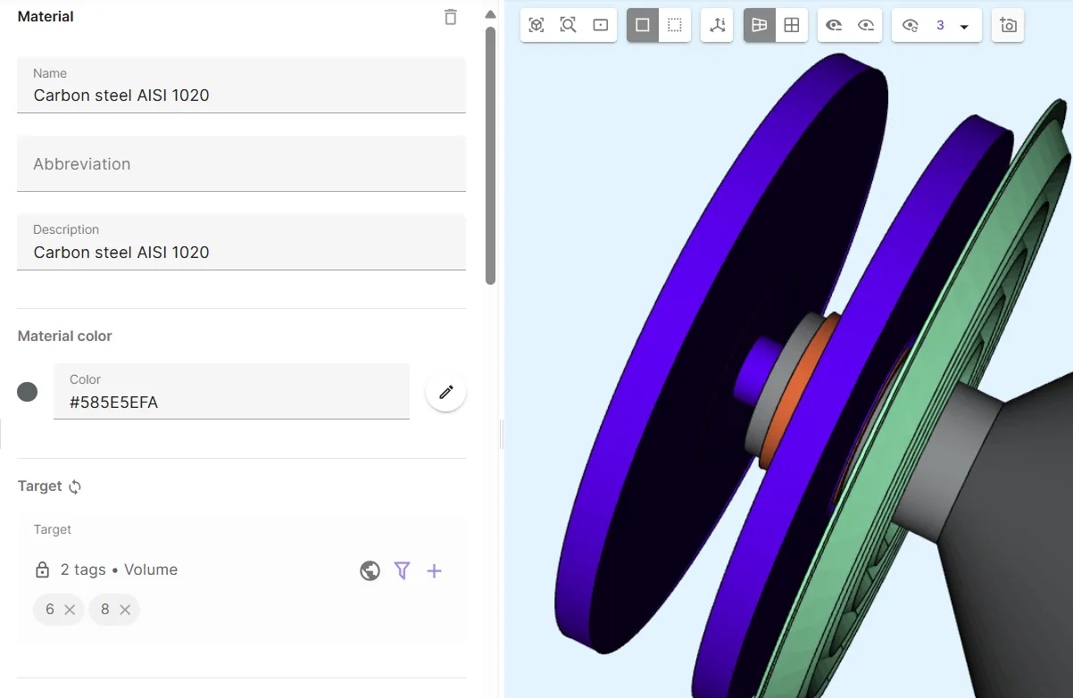
Material 6 - Carbon steel

Assign the Carbon steel AISI 1020 material to the pole piece of the loudspeaker driver.

Your model materials are now defined.

Step 3 - Define the physics

Proceed to the Physics section to define the physics.

In this example, the Solid mechanics, Current flow, Magnetism A and Acoustic waves physics are required. Add all of them under Physics first, and after that, move on to setting up interactions for each physics as below.

Physics 1 - Solid mechanics

• As solid mechanics target, select all volumes except the air bubble.

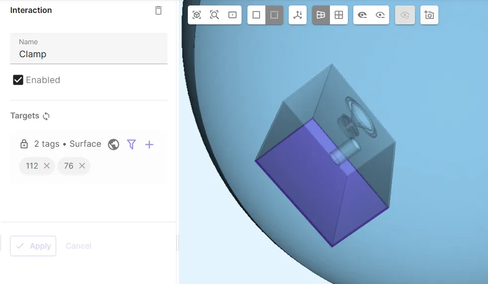
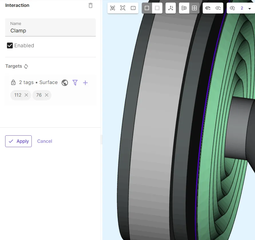
• Add Clamp.

  • As clamp target, select the cabinet bottom surface and the spider edge surface.

    Parallel projection for zooming

    For zooming into small details to pick geometric entities, it can be much easier to use the parallel camera projection. Experiment with the perspective and parallel camera projections liberally to see which works best!

• Add Clamp 2.

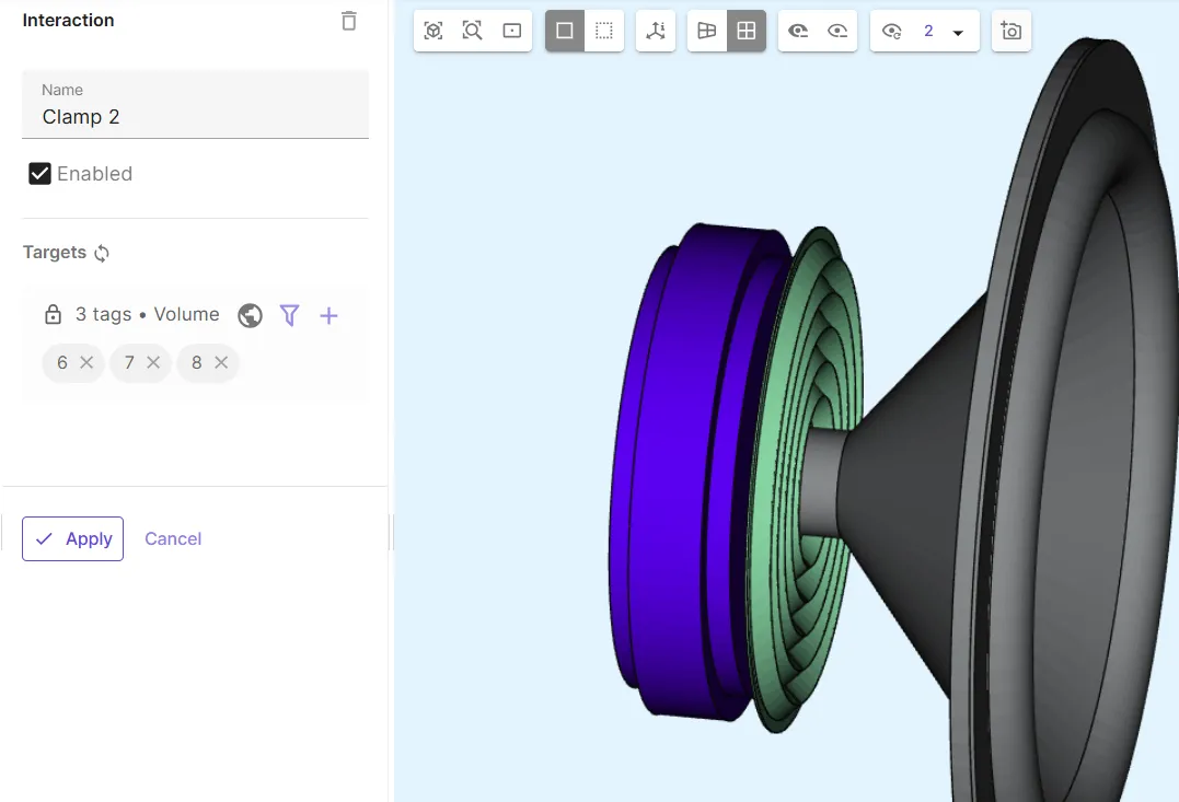
  • As clamp 2 target, select the magnet and driver pole volumes.

• Add Magnetic force to couple Solid mechanics with Magnetism A.

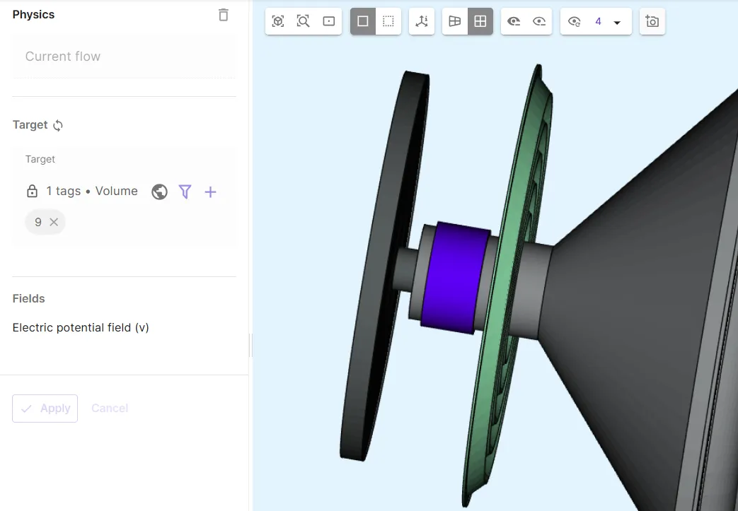
Physics 2 - Current flow

• As current flow target, select the coil volume.
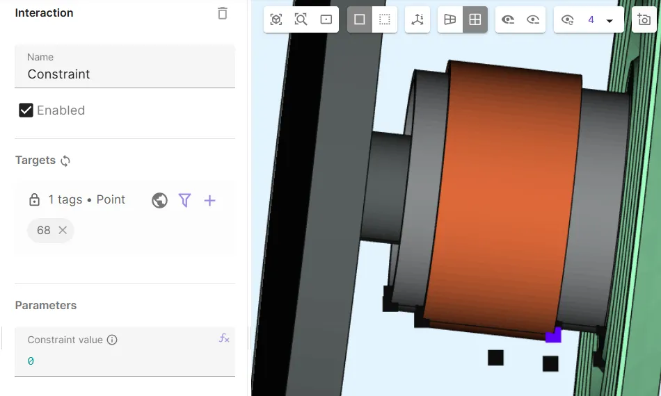
• Add Constraint.
  • As constraint target, select a point on the coil outer boundary.
  • Set constraint value to 0.
• Add Lump V/I cut.
  • As lump V/I target, select a curve on the coil outer boundary.
  • Set Current to 1 + sin(2*pi*freq*t) * 1e-3.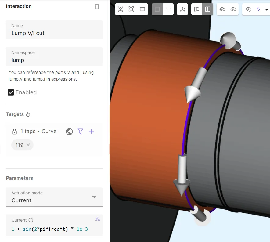

Physics 3 - Magnetism A

• Let magnetism A target default to the whole geometry.
• Add Magnetic wall.
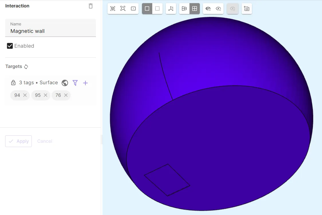
  • As magnetic wall target, select all outer boundary surfaces of the model.
• Add Remanence, which is the permanent magnetic field strength applied on the magnet.
  • As Target, select the magnet volume.
  • Set Remanence (X; Y; Z) as [0; 0.7; 0].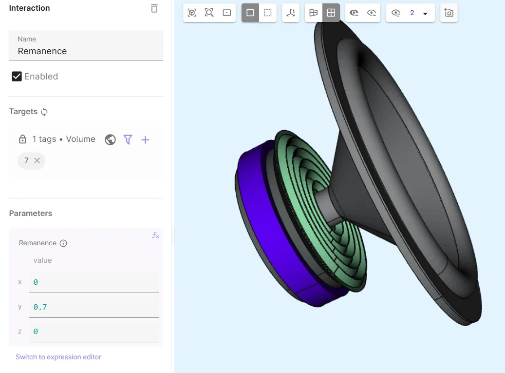
• Add A-v coupling to couple Magnetism A with Current flow.

Physics 4 - Acoustic waves

• As acoustic waves target, select the air bubble volume.
• Add Perfectly matched layer.
  • As Target, select the air bubble outer dome surface.
• Add Acoustic structure to couple Acoustic waves with Solid mechanics.

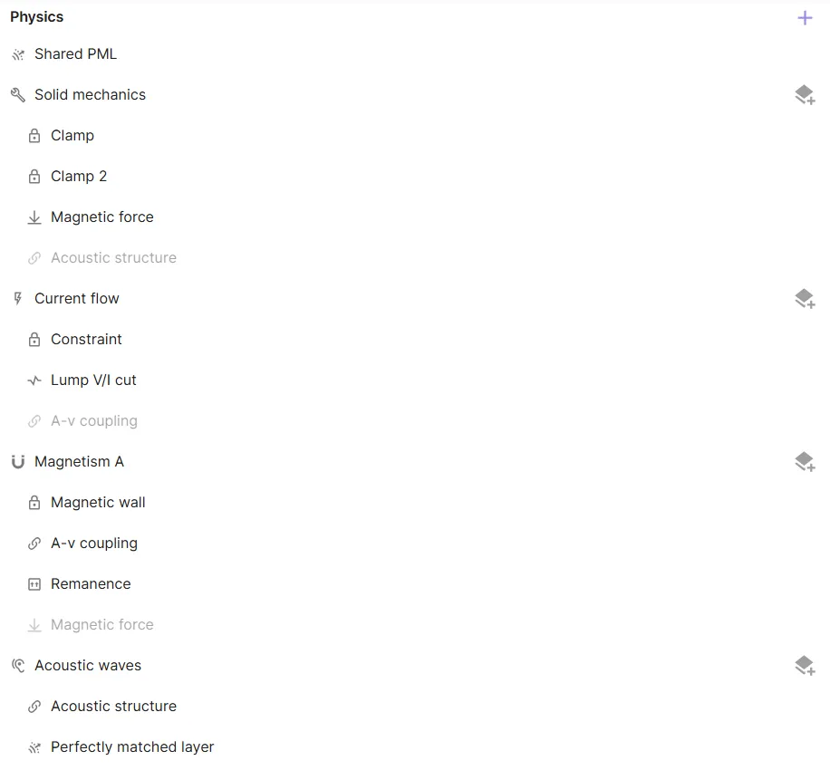
Your simulation physics are now defined, and your physics tree should contain all physics as in the image below.

Step 4 - Generate the mesh

Go to the Simulations section and create a new mesh:

1. Open the collapsible menu for Mesh element size.
2. Set Max size to 0.05.
3. Set Scale factor to 0.5.
4. Apply the settings & mesh.

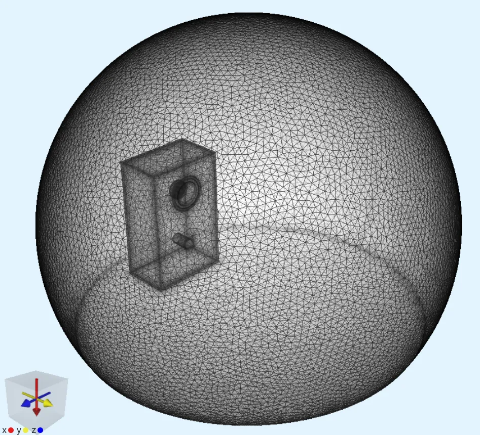
In translucent mode, your mesh should look something like in the image below:

Step 5 - Simulate

In the Simulations section, create a new simulation:

• In Simulation settings:
  • Set Analysis type to Multiharmonic.
  • Set Fundamental frequency to 3e3.
  • Set Harmonics to 1 2 3.
  • Set Solver mode to Iterative solver.
• In Mesh, select the mesh you created.
• In Inputs:
  • Add freq sweep.
    • Set Override expression to [100, 500, 1e3, 3e3, 5e3, 8e3, 10e3, 15e3, 20e3].
• In Outputs:
  • Add the p, B and u harmonic field outputs.
  • Add a custom value output called SPL.
    • Set Output expression to integrate(reg.air_target, p, 3).

Run the simulation and plot/visualize results.

Large main node recommended

With a large mesh such as here, a large main node with 16 or 32 CPUs is beneficial.

Results

Here, the pressure field p is visualized. A roughly human-sized mannequin is added in front of the loudspeaker to visualize acoustic waves interpolated on the surface of the body.

Visualizations & post-processing

The animation above, as well as the speaker driver visualization in Overview were made using Paraview. The post-processing tools in Allsolve are still limited, so external software is recommended for more sophisticated post-processing, such as animations.

Footnotes

1. Dr. Abhishek Deshmukh. Acoustics simulations powered by the cloud. Quanscient webinars (2024). https://quanscient.com/events/acoustics-webinar/register ↩