
Twisted superconductor AC Loss - SC 002
In this tutorial, AC loss in a high-temperature superconducting (HTS) wire is simulated using the H-φ formulation.
Model definition
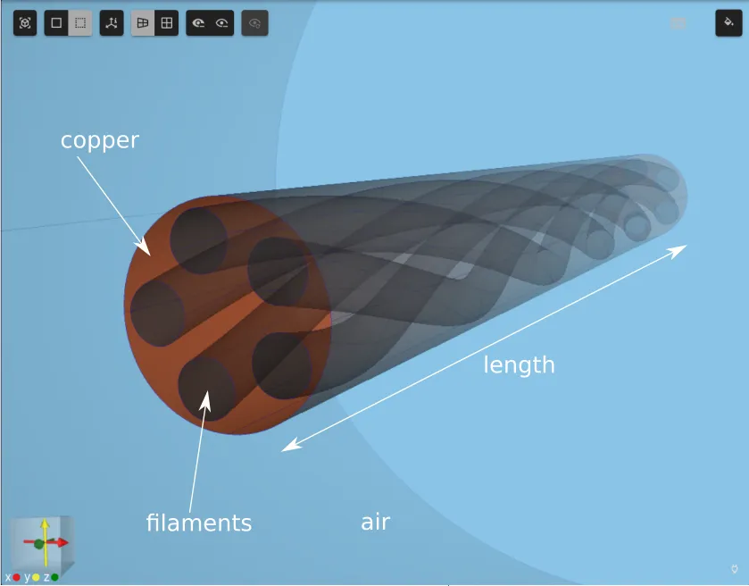
Section titled “Model definition”The wire consists of twisted superconducting filaments embedded into a copper matrix. The whole modelling domain with an air cylinder around the wire is illustrated below.
| Element | Dimension |
|---|---|
| Air cylinder diameter | 10 mm |
| Copper cylinder diameter | 535 μm |
| Filament diameter | 350 μm |
| Domain length | 10 mm |
Output results
Section titled “Output results”- Joule losses as a function of time in the copper and the superconducting filament regions. The losses over the volume of interest can be computed as
Material Data
Section titled “Material Data”Magnetic permeability, :
- all domains:
Electric resistivity, :
- Copper:
- Superconducting filaments:
-
- Critical electric field strength,
- Exponent,
- Critical electric current,
- Total cross-section are of superconducting filaments,
- Critical electric current density,
-
Source
Section titled “Source”The problem is sourced by applying a total current of
where the frequency is .
Step-by-step guide
Section titled “Step-by-step guide”Here you’ll find a detailed step-by-step tutorial on how to simulate AC loss in a twisted filament HTS wire Quanscient Allsolve.
Step 1 - Import the geometry
Section titled “Step 1 - Import the geometry”-
Start with a new project and name it as
SC twisted filament AC loss -
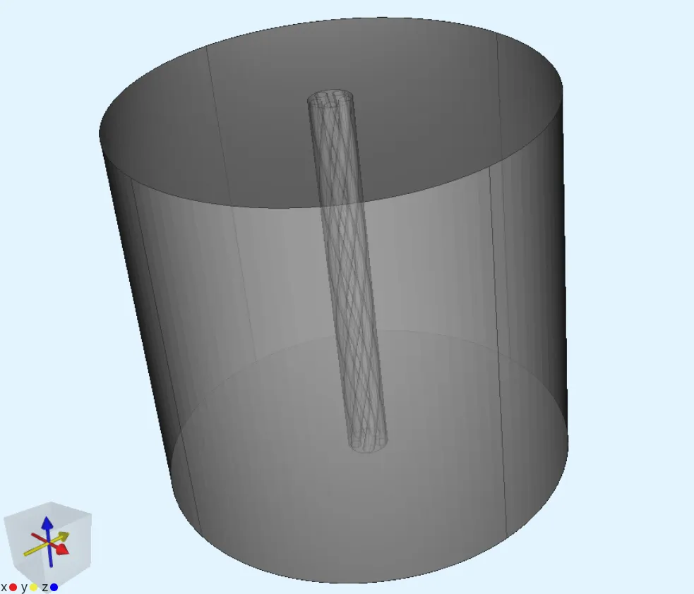
Import the geometry as a
.stepfile with default import options.File download link: twisted-superconductor.step
-
Confirm model changes.
Step 2 - Define regions
Section titled “Step 2 - Define regions”-
Go to the
Commonsidebar. -
Define a region for air:
Region name Region type Target airVolume Air cylinder 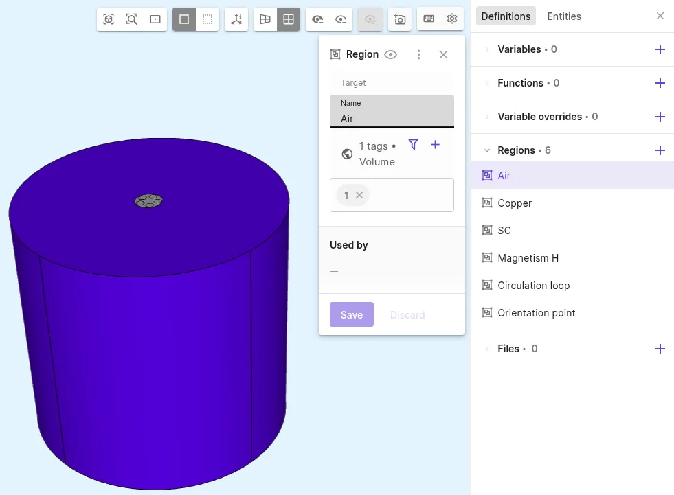
-
Define a region for copper:
Region name Region type Target copperVolume Copper matrix 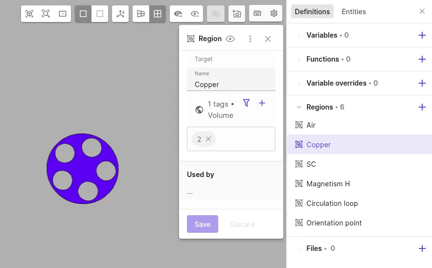
-
Define a region for the superconducting filaments:
Region name Region type Target scVolume SC filaments 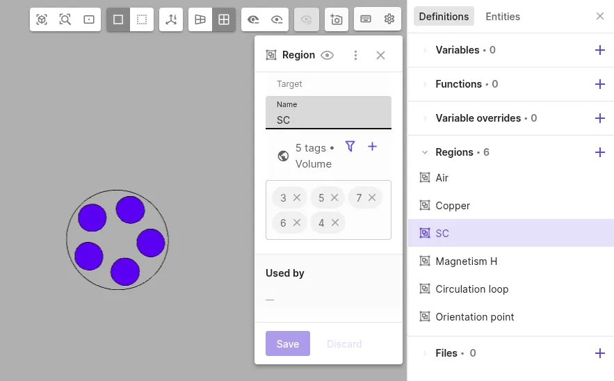
Step 3 - Define materials
Section titled “Step 3 - Define materials”-
Assign the Air material to the
airregion: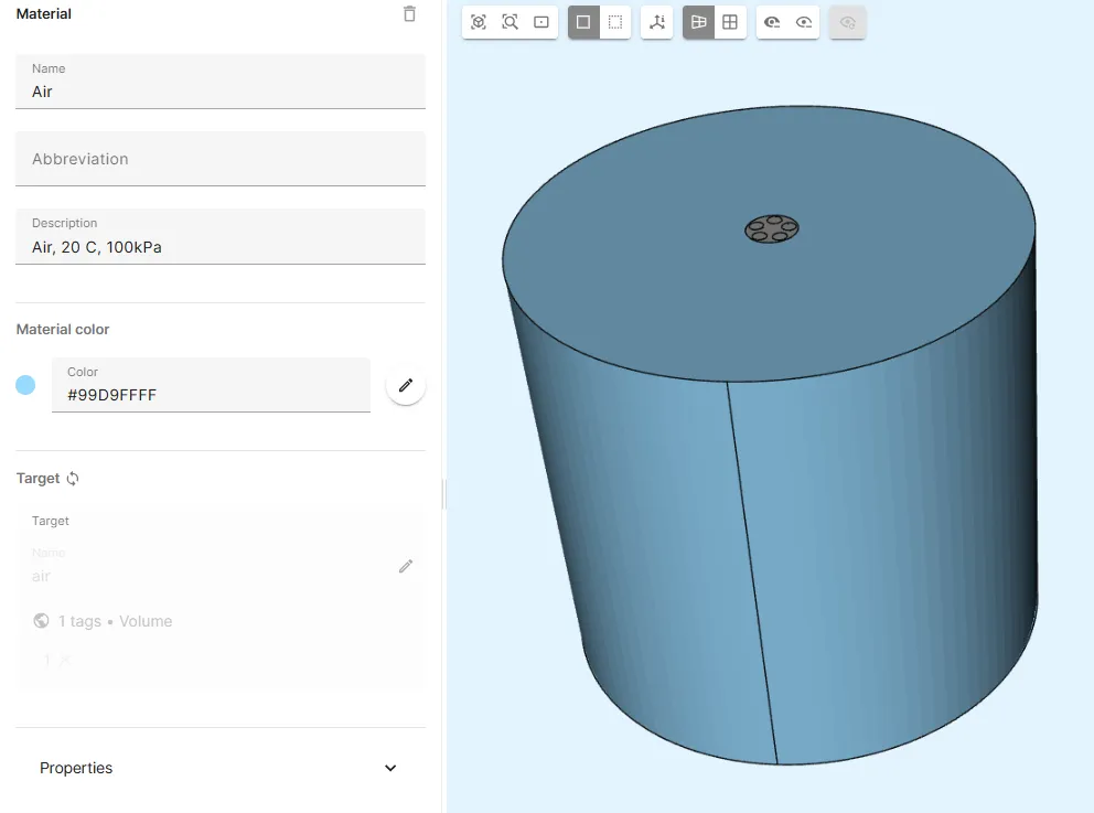
-
Assign the Copper material to the
copperregion: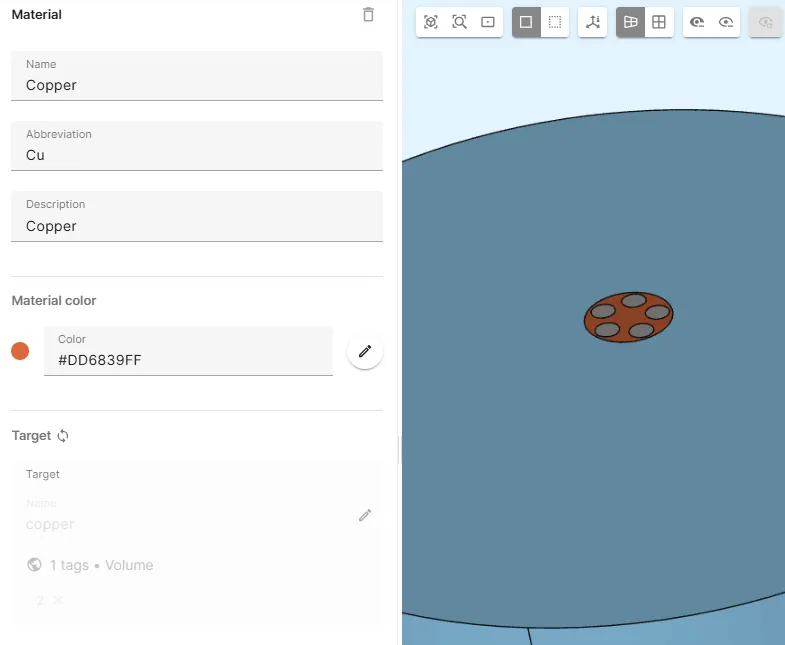
-
Assign the YBCO superconductor material to the
scregion: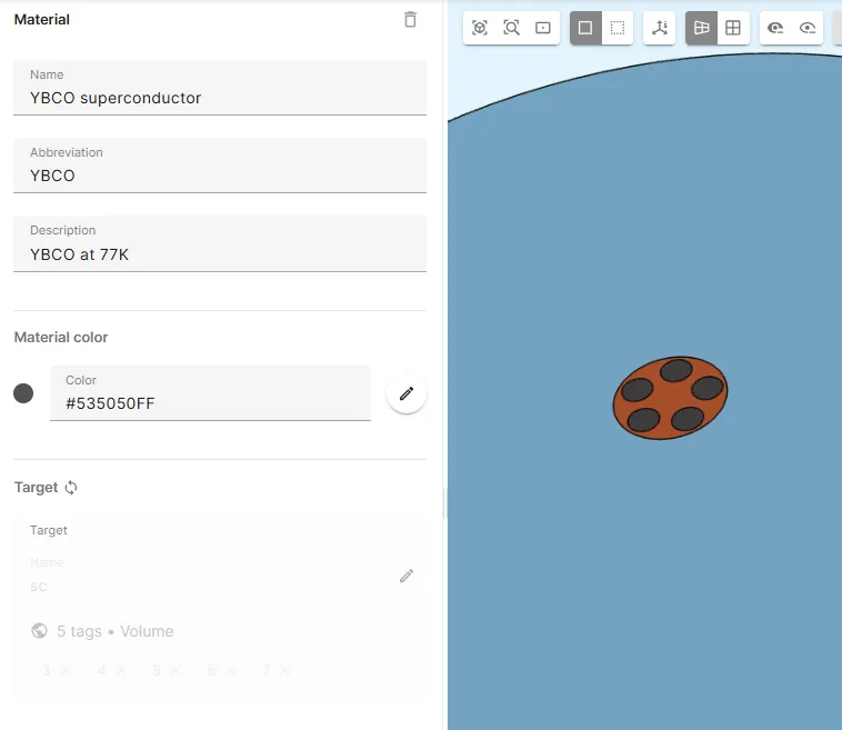
Step 4 - Define variables
Section titled “Step 4 - Define variables”-
Define new variables:
Name Description Expression f Frequency [Hz] 50YBCO_Ic Critical current [A] 100YBCO_Asc Filament cross-section area [m^2] 3.4541e-7Iop Operating current [A] 0.8 * YBCO_Ic * sin(2 * pi * f * t) -
Modify existing variables:
Name Modified expression YBCO_Jc YBCO_Ic / YBCO_AscYBCO_n 30
Step 5 - Define physics and apply the current source
Section titled “Step 5 - Define physics and apply the current source”-
Go to the
Physicssection. -
Add the
Magnetism Hphysics:Physics Target Magnetism H Copper matrix and SC filaments 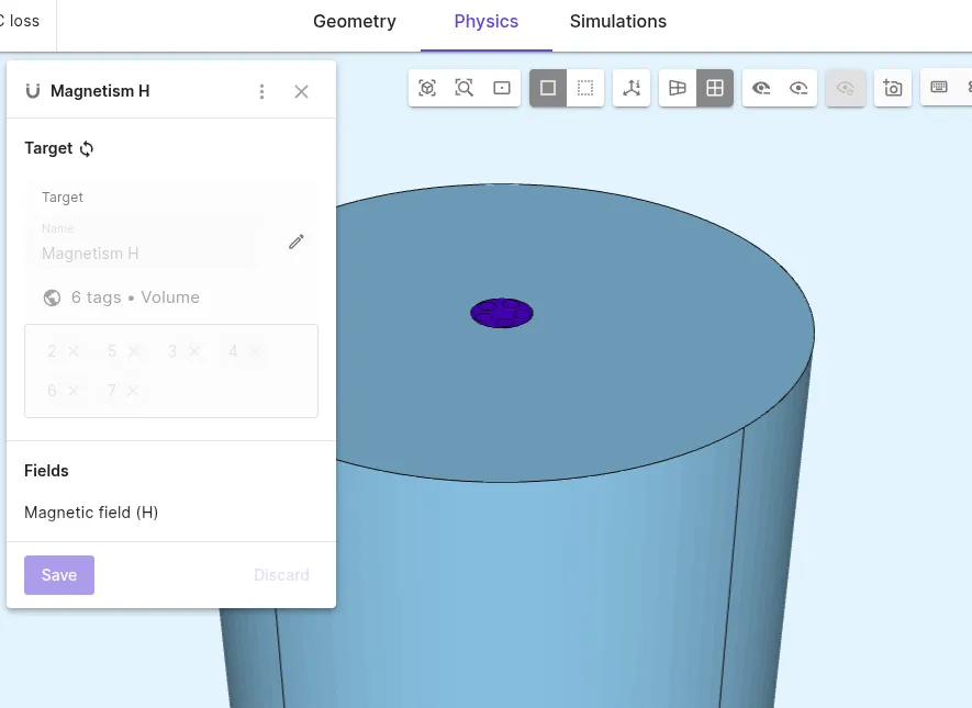
-
Add the
Magnetism φphysics:Physics Target Magnetism φ Air cylinder ( airregion)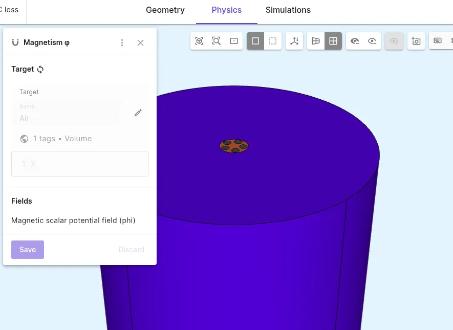
-
Add a
Lump I/V cutinteraction to Magnetism φ.Interaction name Interaction type Target Value Current source Lump I/V cuta counter-clockwise loop at the top edge of the copper matrix Iop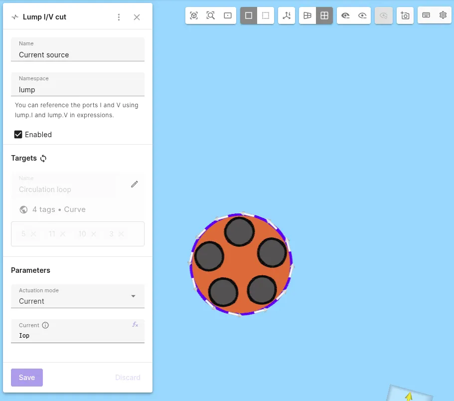
-
Add a
Constraintinteraction to Magnetism φ:Interaction name Interaction type Target Value Gauge Constrainta point at the external boundary of the air domain 0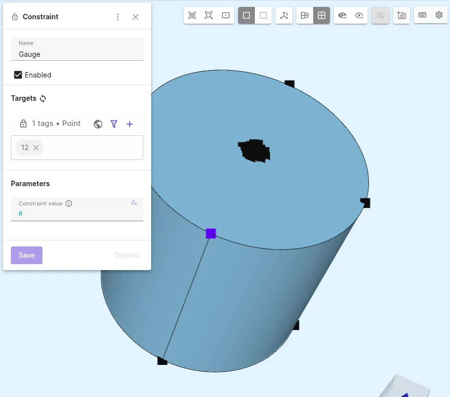
-
Add the
H-φ couplinginteraction to Magnetism H. -
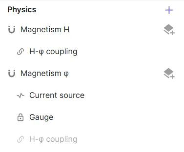
Before moving on, check that your physics tree matches the one below:
Step 6 - Generate a mesh
Section titled “Step 6 - Generate a mesh”-
Go to the
Simulationssection. -
Add a new mesh.
-
Set Autorefine to
Disabled. -
Open the collapsible menu for
Mesh element size. -
Set Curvature enhancement to
25. -
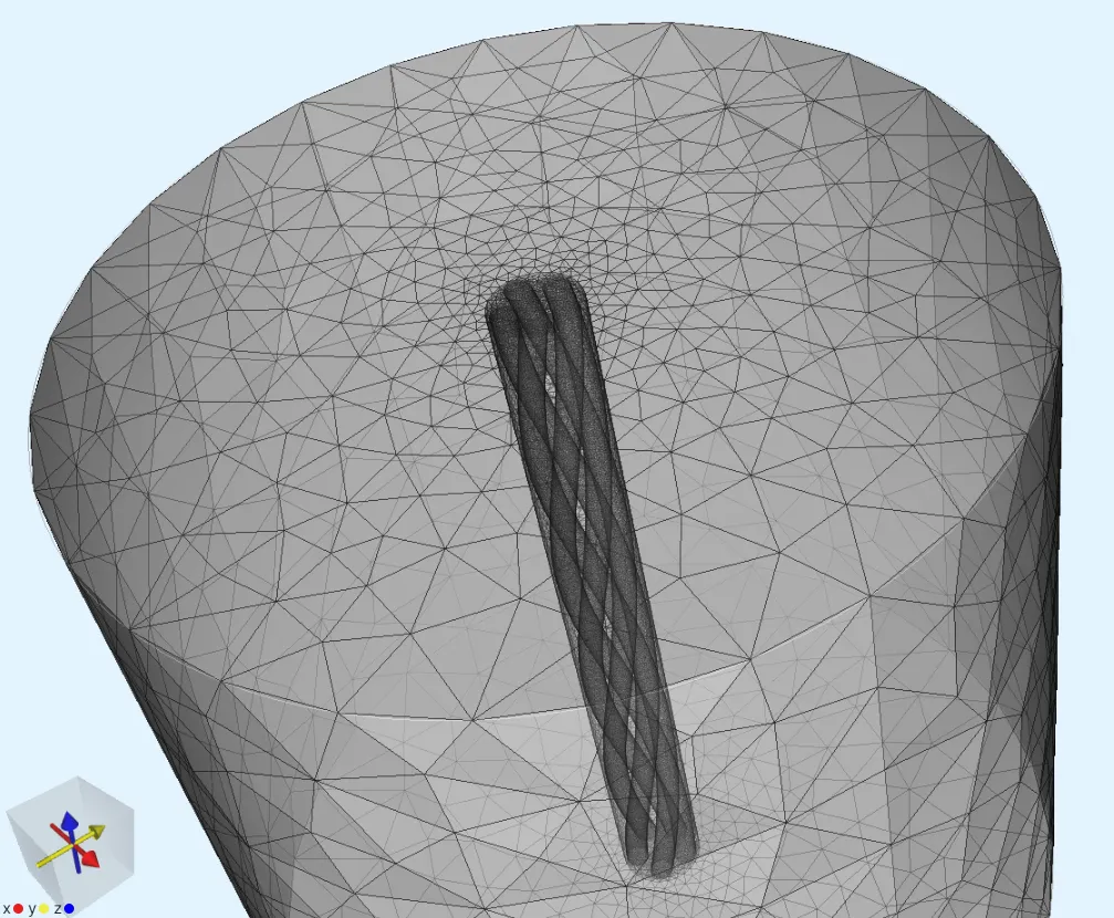
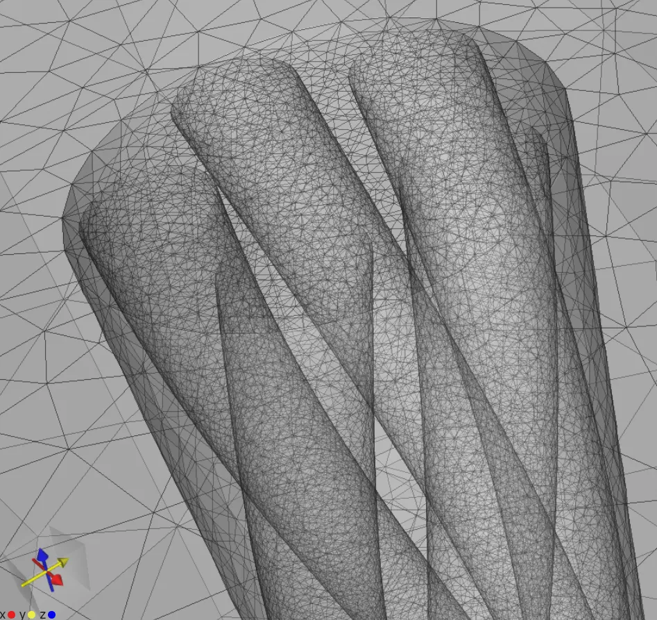
Generate the mesh and check the preview.
Step 7 - Select simulation settings
Section titled “Step 7 - Select simulation settings”-
Add a new simulation.
-
Set Analysis type to
Transient. -
Select Transient settings:
Timestep algorithm Start time [s] End time [s] Timestep size [s] Implicit Euler 00.010.0001 -
Set Solver mode to
Iterative solver. -
Set Node count to
50. -
Select
Mesh 1as the mesh for your simulation. -
Define custom value outputs for computing Joule losses in the filaments and copper:
Output name Output type Output expression SC loss Custom value output integrate(reg.sc, transpose(E) * j, 4)Cu loss Custom value output integrate(reg.copper, transpose(E) * j, 4) -
Open the Script for your simulation.
-
Enable
Scripting mode. -
Replace the first autogenerated line under
# Magnetism Hwith the following Newton-linearization [4]:rho = 1/par.sigma(df.j)dedj = rho*qs.eye(3) + (expr.YBCO_n-1.0)*rho/qs.max(df.j*df.j, 1e-40) * df.j * qs.transpose(df.j)dofe = rho*df.j + dedj * (qs.curl(qs.dof(fld.H))+var.curl_dof_Hs - qs.curl(fld.H)-var.curl_Hs)form += qs.integral(reg.sc, dofe * (qs.curl(qs.tf(fld.H)) - var.curl_tf_Hs))form += qs.integral(reg.copper, qs.inverse(par.sigma(df.j)) * (qs.curl(qs.dof(fld.H)) + var.curl_dof_Hs) * (qs.curl(qs.tf(fld.H)) - var.curl_tf_Hs))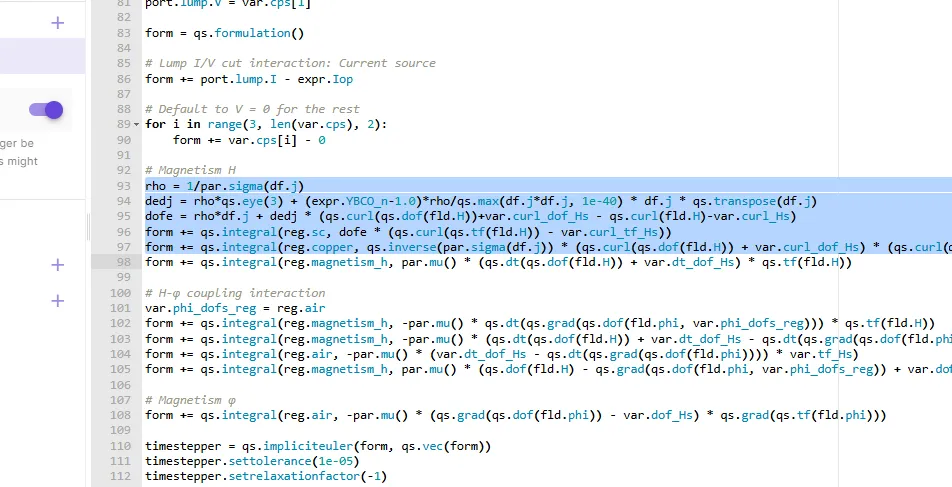
Step 8 - Run the simulation and see results
Section titled “Step 8 - Run the simulation and see results”-
Run the simulation.
-
To follow the simulation progress, open
Logs. -
The SC and Cu loss results can be seen in
Plotting, even while the simulation is running: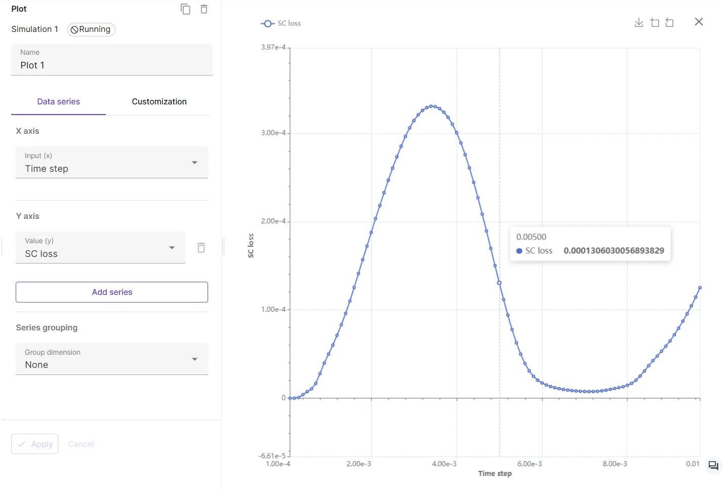
References
Section titled “References”[1] H-φ Formulation in Sparselizard Combined With Domain Decomposition Methods for Modeling Superconducting Tapes, Stacks, and Twisted Wires. https://doi.org/10.1109/TASC.2023.3240389
[2] Allsolve demo project of Superconductor AC losses. https://allsolve.quanscient.com/#/projects/demo/8fed82d1-5bf0-4c02-835b-94e65a60f847
[3] Youtube tutorial of Superconductor AC losses. https://youtu.be/B9QZZ5y7RpQ
[4] Newton Linearization. https://en.wikiversity.org/wiki/Nonlinear_finite_elements/Newton_method_for_finite_elements