
Plotting simulation results
Plotting turns simulation value outputs into interactive charts. Plots live under Results in the simulation tree and can be created while a simulation is still running.
To add a plot, select + next to Plotting:
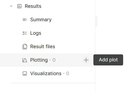
Each plot starts with one empty Data series. A single plot can contain multiple series. Select Save in the plot settings footer to apply changes.
Plot settings are split into two tabs:
| Tab | Purpose |
|---|---|
| Basic | Plot name, Chart type, and Data series configuration |
| Customization | Axes, color scale, chart-specific options, and series styling |
Chart types
Section titled “Chart types”Select Chart type on the Basic tab. The dimension labels on each series change to match the selected type.
| Chart type | Dimensions | Typical use |
|---|---|---|
| Cartesian | X value, Y value, Color value (optional) | Time histories, sweeps, general XY plots |
| Polar | Angle (θ), Radius (r), Color value (optional) | Radiation patterns, angular sweeps |
| Heatmap | X value, Y value, Color value (required) | Two-dimensional parameter maps |
| 3D | X value, Y value, Z value, Color value (optional) | Three-variable relationships |
| Smith | Magnitude, Phase, Color value (optional) | RF reflection and impedance analysis |
Supported Series type options depend on the chart type:
| Chart type | Series types |
|---|---|
| Cartesian | Line, bar, scatter |
| Polar | Line, scatter, bar |
| Heatmap | — (no series type; data is binned into a grid) |
| 3D | Scatter, bar |
| Smith | Line, scatter |
3D plots always use canvas rendering. Other chart types can use Canvas or SVG under General > Plot rendering.
Cartesian
Section titled “Cartesian”The default chart type. Use Right axis on a series (series menu or Customization > Series) to plot that series on a separate Y scale. Configure the left Y scale under Y value; the right Y scale under Tertiary axis.
Map one output to Angle (θ) and another to Radius (r). Optional Color value adds a color bar. The angle axis is always linear; set its unit with Degrees / Radians below.
Under Polar settings in Customization:
| Setting | Description |
|---|---|
| Start angle | Angle at the top of the chart (degrees) |
| Direction | Clockwise or Counter-clockwise |
| Degrees / Radians | Unit of the angle data |
| Radiation pattern preset | Applies common defaults for antenna radiation patterns |
Heatmap
Section titled “Heatmap”Requires X value, Y value, and Color value. Data is grouped into bins; cell color represents the averaged color value in each bin. With a logarithmic axis scale, bins are spaced evenly in log space and labeled with the original values.
A heatmap shows a single data series. Add series, Series from, Right axis, and Customize are not available, and switching an existing plot to Heatmap keeps only its first series.
Requires X value, Y value, and Z value. Rotate the view by dragging in the chart area. Optional Color value maps point or bar color.
Bar series on 3D plots use the Color scale settings for coloring.
Requires Magnitude and Phase outputs, for example S-parameter magnitude and phase from an RF simulation. The chart shows the reflection coefficient locus on a Smith grid. The dimension labels follow the selected units, for example Magnitude (linear) or Magnitude (dB) and Phase (°) or Phase (rad).
Each series can also set a Frequency column, the output shown as frequency in the tooltip. Because it is set per series, series from different data sources (for example a simulation and a CSV file) can use their own frequency columns. Optional Color value colors the locus using the Color scale settings.
Under Smith chart in Customization:
| Setting | Description |
|---|---|
| Reference impedance Z₀ (Ω) | Characteristic impedance for impedance and admittance readouts (default 50 Ω) |
| Magnitude unit | Linear or dB magnitude input data |
| Phase unit | Degrees or Radians phase input data |
| Impedance circles | Toggle constant-resistance circles (on by default) |
| Admittance circles | Toggle constant-conductance circles (off by default) |
| VSWR circle | Draw a circle at a specified VSWR value (1 or greater) |
| Grid lines / Minor grid lines | Toggle Smith grid lines (both on by default) |
| Label font size | Font size for axis tick labels |
Hover a point to see reflection coefficient (|Γ| in dB), impedance, admittance, and VSWR values in the tooltip, plus frequency when the series has a Frequency column.
Data series
Section titled “Data series”Each entry under Data series defines one plotted dataset. Expand a series to configure it.
| Setting | Description |
|---|---|
| Data source | This simulation (default), another simulation in the project, or a CSV file uploaded as an extra input file |
| Dimension fields | Values assigned to the chart axes (labels depend on Chart type; see table above) |
| Series from | Optional. Available when data has more than two free dimensions. Groups rows by a dimension (for example Sweep or Time) and creates one series per group |
| Frequency column | Smith charts only. Optional output shown as frequency in the tooltip |
| Bound input | Optional. Available when data has more than three dimensions. Fixes a dimension — for example Array index (0, 1, 2…) to plot one element of an array output |
| Include | When Series from is set, limits which groups are plotted |
Use Add series to plot multiple outputs on the same chart (not available for heatmaps). Open the series menu (⋯) to Rename, Customize, assign Right axis, or Delete a series.
Axes and scales
Section titled “Axes and scales”Axis settings appear under Customization for chart types that use continuous axes. Panel titles match the plot dimension — for example X value and Y value on Cartesian charts, Angle (θ) and Radius (r) on polar charts, and Z value on 3D charts.
| Panel | Cartesian | Polar | 3D |
|---|---|---|---|
| First panel | X value | Angle (θ) | X value |
| Second panel | Y value | Radius (r) | Y value |
| Third panel | Tertiary axis (right Y, when used) | — | Z value |
Smith charts use Smith chart settings instead of separate axis panels.
Common options within each axis panel:
| Setting | Description |
|---|---|
| Scale | Linear, Logarithmic, dB, or dB (normalized). The polar Angle (θ) axis supports only Linear |
| Min / Max | Manual axis bounds; leave empty for automatic range |
| Override label | Custom axis title |
| Number format | Tick label format: auto, scientific, fixed, engineering, or SI prefix |
| Split lines | Major and minor grid lines |
| Align ticks with left axis | Align right-axis ticks with left-axis ticks (dual Y plots) |
Logarithmic scale requires the plotted values on that axis to be either all positive or all negative. Zero values in otherwise positive data are left out of the plot. Mixed-sign data, or data without a non-zero range, shows a configuration message instead of the chart.
Color scale
Section titled “Color scale”The Color scale panel appears when the chart uses color mapping:
- Heatmap — always
- 3D bar series
- Cartesian, Polar, Smith, or 3D plots when Color value is set on a series. Line series are drawn with a color gradient along the line
| Setting | Description |
|---|---|
| Color map | Sequential, Cool-Warm, Grayscale, or Hot |
| Scale | Linear, dB, or dB (normalized) applied to the color values |
| Min / Max | Clamp the color range; leave empty to span the data |
Drag or hover on the color bar below the chart to highlight corresponding data points.
Series styling
Section titled “Series styling”Under Customization > Series, select Configured series to style one series or All series for shared settings.
| Setting | Description |
|---|---|
| Series type | Line, bar, or scatter (where supported) |
| Line style / Line width / Point size | Line appearance (line series) |
| Smoothness | Line smoothing (line series) |
| Connect over nulls | Draw through missing data points instead of breaking the line |
| Right axis | Plot on the right Y scale (Cartesian) |
| Automatic color | Use the default series color or pick a fixed color |
| Legend format | Template for legend entries when Series from grouping is active |
General settings
Section titled “General settings”Under Customization > General:
| Setting | Description |
|---|---|
| Plot title / Plot subtitle | Chart heading text |
| Align title center | Center the title over the plot area |
| Plot rendering | Canvas (performance) or SVG (sharp exports) |
| Legend display | Position: none, top, or right; style and font size |
| Show toolbox | Zoom and save-image controls on the chart |
To export a crisp image, set Plot rendering to SVG, then use Save image in the chart toolbox.
Chart toolbox
Section titled “Chart toolbox”When Show toolbox is enabled, the chart toolbar provides:
- Zoom — zoom into a region; Zoom reset restores the full view
- Save image — download the chart as PNG
Cartesian plots also support scroll-wheel zoom on the axes. Heatmap, 3D, and Smith charts do not use axis zoom in the same way.
Large datasets
Section titled “Large datasets”To keep plots responsive, series with more than 10,000 points are reduced before rendering:
- Line series are downsampled. The peaks and the full data range are kept.
- Scatter series are thinned so that overlapping points are drawn only once.
- Bar series and all 3D series cannot be reduced and are not rendered automatically.
A notice on the plot shows how many points are displayed. Select Show all and confirm to render every point. Rendering all points can make the plot and the application slow. The setting resets when you select a different plot.