Shared expressions
Quanscient Allsolve makes use of public variables called shared expressions, that are visible in the scope of a project. This means that once you have defined a shared expression, it can be used in all sections of the application.
You can see symbols in various places that serve as a reminder to the user:
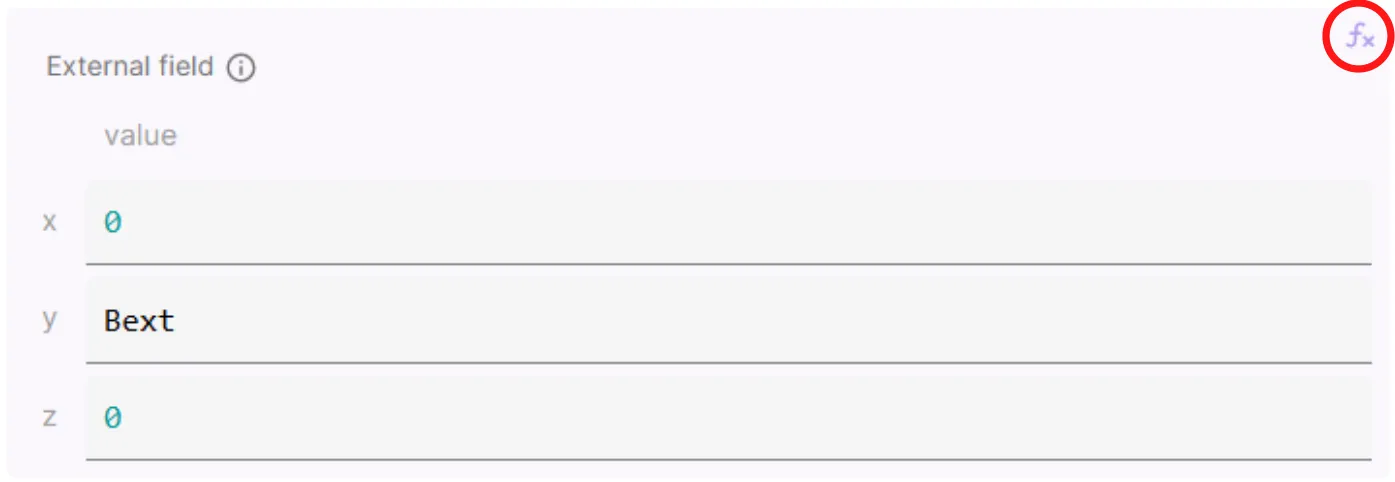
Wherever you see an symbol, shared expressions can be used.
In the image above, shared expression Bext is used to define external magnetic flux density in the Y-direction.
Shared expressions are defined in the Properties section. They have 3 parameters:
- Name
- A short but descriptive name, by which the shared expression is referred to.
freqBext
- A short but descriptive name, by which the shared expression is referred to.
- Description (optional)
- A description of the shared expression in a few words, along with the unit.
Fundamental frequency [Hz]Magnetic flux density of the external field [T]
- A description of the shared expression in a few words, along with the unit.
- Expression
- The mathematical expression by which the shared expression is defined.
- An expression can consist of:
- numbers in integer, double or scientific format (
42,-1.72901,1.2e-18) - other shared expressions
- basic algebraic operators (
+,-,*, …) - basic math constants (
pi,mu0, …) - built-in variables (
t,x, …) - predefined functions (
sin,exp, …)
- numbers in integer, double or scientific format (
To see an exhaustive list of built-in shared expressions and further technical details, see Expressions.
Use-cases
Shared expressions can be utilized in many different areas in projects. These include:
- Creating geometries
- Setting up material properties
- Setting up physics interactions
- Overriding other shared expressions
- Using shared expressions for parametric sweeps
- Defining custom value outputs
Below are some general points and practical examples for each of these use-cases.
Creating geometries
Shared expressions can be very useful for parametrization during modeling.
If you want to model an object with known dimensions, you can start out by inputting them as shared expressions, and then move on to modeling. If there is a need to later modify the model dimensions, you can simply edit your shared expressions and rebuild the model.
Example: CMUT membrane disc
- CMUT membrane thickness and radius are defined as shared expressions
thmemandradmem: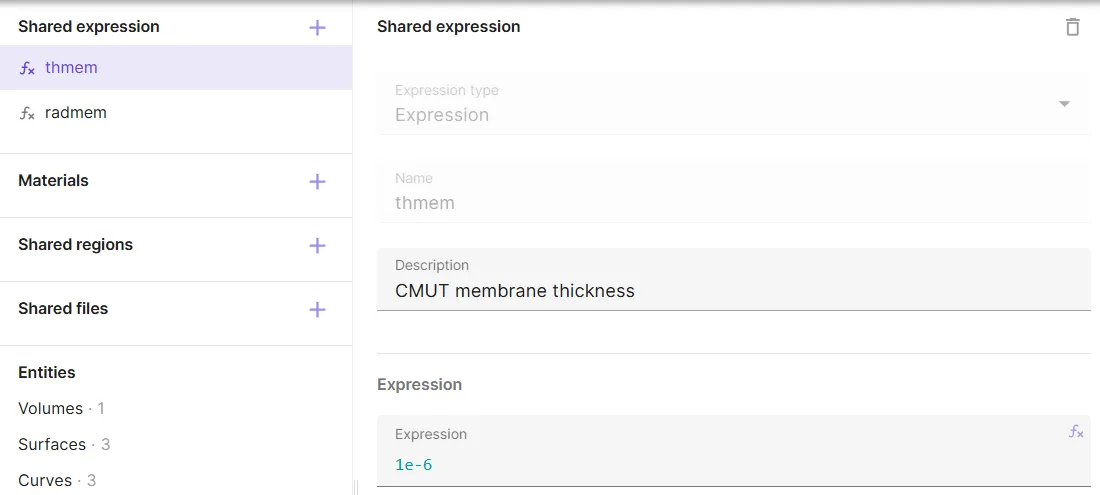
thmemandradmemare used to create the CMUT membrane disc: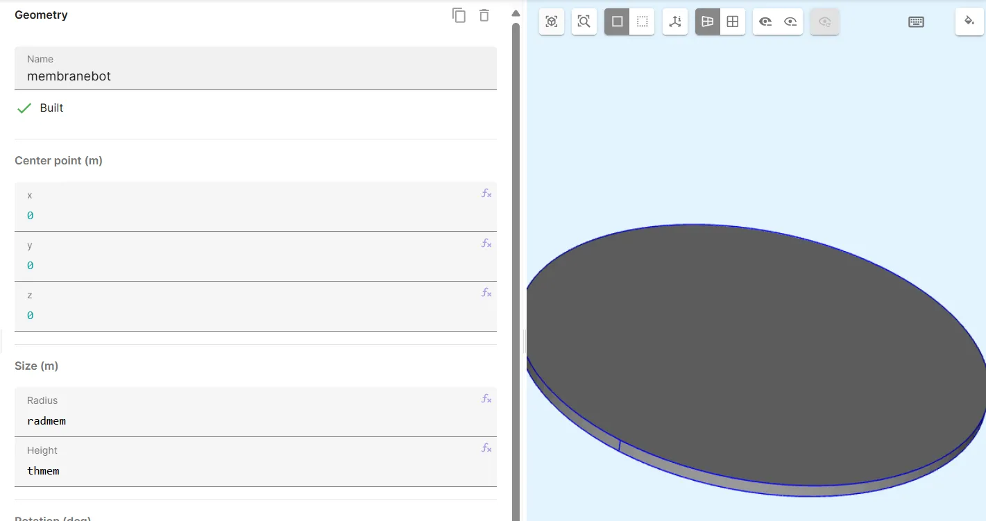
Source: CMUT example case
Material properties
Material properties can be defined using shared expressions, be it setting up properties for a new material, or modifying a predefined material. Material properties can then later be modified through the shared expressions.
Example 1: Clamped-clamped beam
- Shared expressions
density,poisson(Poisson’s ratio) andyoung(Young’s modulus) are defined. density,poissonandyoungare used to define theDensityandElasticity matrixmaterial properties: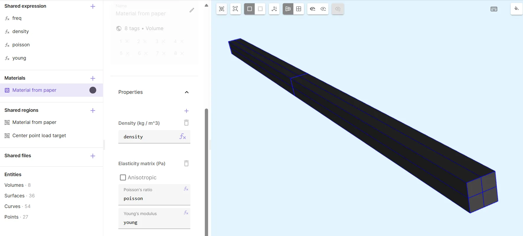
Source: Backbone curve of a clamped-clamped beam
Example 2: YBCO Quench
- The superconducting
YBCOmaterial is added. Shared expressions are automatically created for the YBCO power law.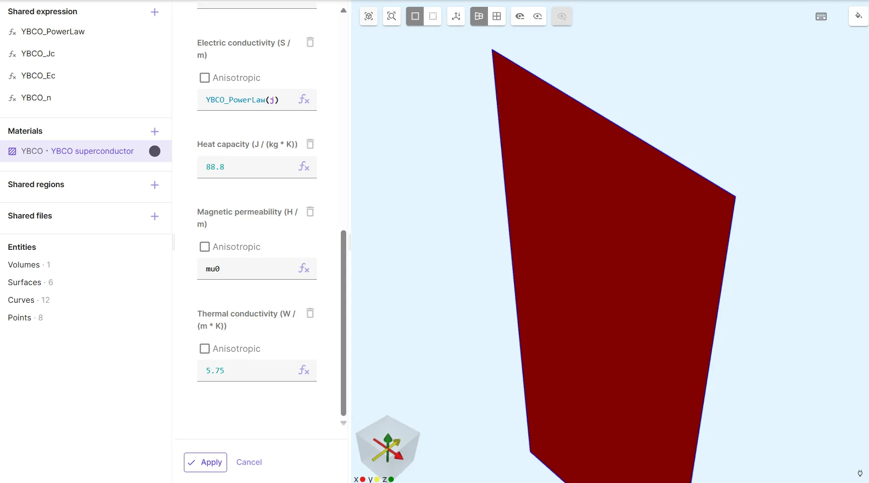
- The current density is automatically defined as a constant,
YBCO_Jc.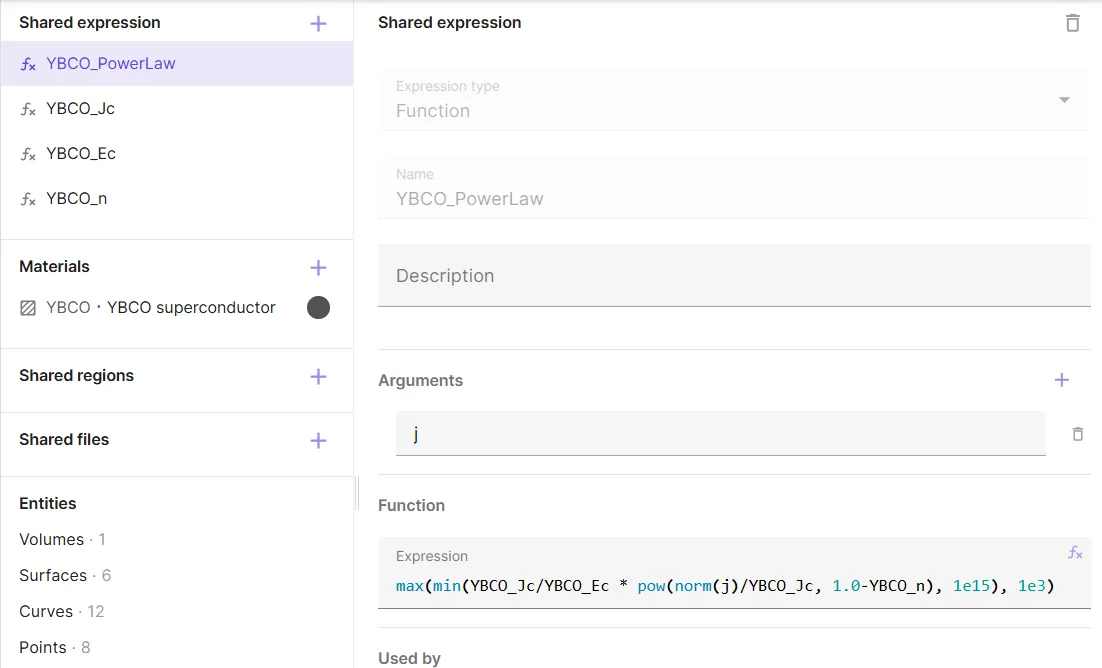
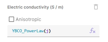
- The
YBCO_PowerLawshared expression is modified, so that the current density is now a function of temperature,Jc(T). TemperatureTand current density functionJcare added as shared expressions.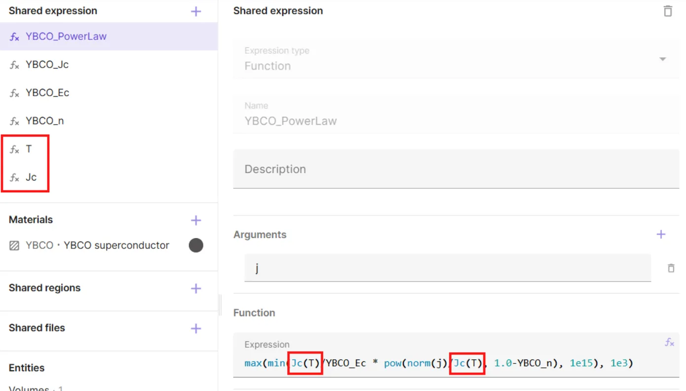
Source: Quench - Hello World Demo
Physics interactions
Many physics interactions can be parametrized using shared expressions.
Example: Steady state heat transfer
- Shared expressions
h(heat transfer coefficient) andTamb(ambient temperature) are defined. - Heat source expression is given as
-h * (T - Tamb):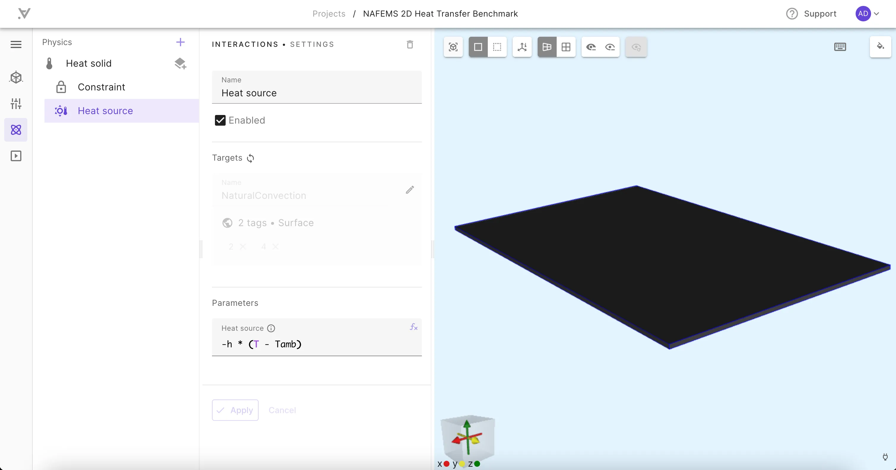
Source: Steady state heat transfer in solid materials - NAFEMS Benchmark
Overriding shared expressions
Sometimes you might want to modify the value of a shared expression in a specific simulation. Allsolve allows you to override a shared expression for the runtime of a simulation. This can be used in sensitivity analysis or debugging, for example, where it is useful to quickly test the effect of changing a single parameter without modifying the original simulation setup.
Parametric sweeps
One of the most powerful applications of shared expressions is in simulation sweeps.
Sweeps are an extension to overrides, and a sweep with a single value as the override expression is identical to an override. Only with sweeps, a vector of values can also be input as the override expression. In this case, a series of simulations is run - one simulation for each override value in the vector.
With sweeps, you can easily run multiple variations of your model in one go, varying one or more parameters. Parameters to be swept must be defined as shared expressions.
Example: MEMS Pull-in analysis
- Direct current voltage is defined as a shared expression,
Vdc. - A
Vdc sweepinput is added to the simulation: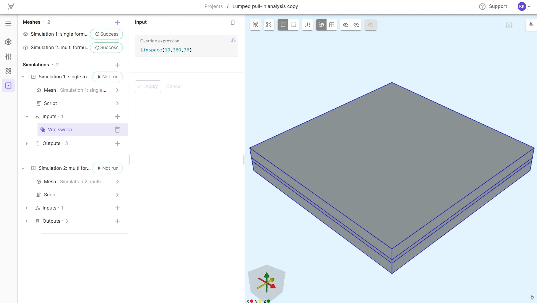
Source: Pull-in analysis of a MEMS device
Custom value outputs
Shared expressions can be used to define custom value outputs, which are single numerical values that can be extracted from your simulation results. Custom value outputs, along with field outputs, are the two main categories of simulation outputs in Quanscient Allsolve.
Using field variables in shared expressions
Field variables, such as displacement field u, current density field j or magnetic flux density field B can be used in shared expressions, but they must be passed on to them as function arguments.
Example: YBCO Powerlaw
When the superconducting YBCO material is added to a project, the YBCO PowerLaw shared expression is automatically created:
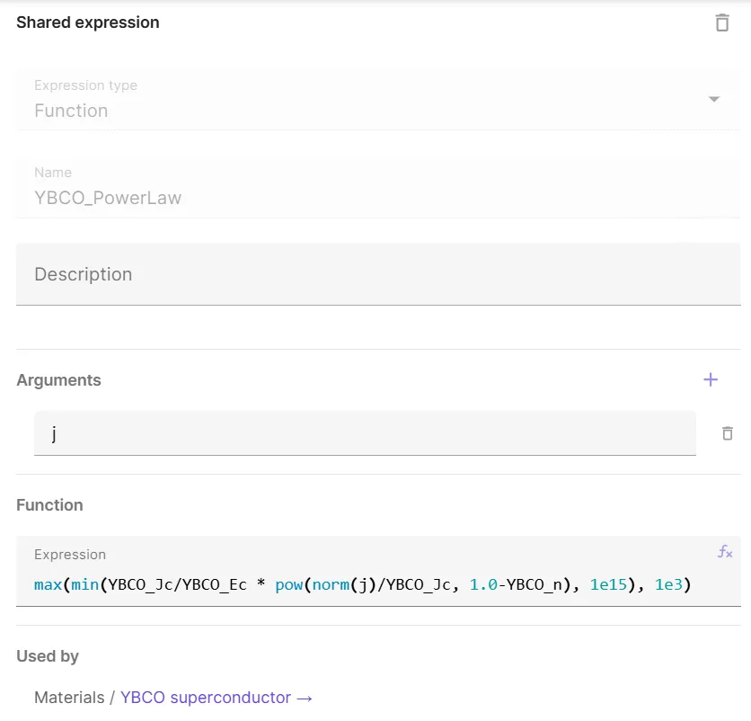
Note, that the Expression type is Function, and the j field is added as an argument.
Now the j field can be passed on to the powerlaw function wherever it is called without causing errors.
The function is called in YBCO material properties like this: