HB 001 - AC Joule heating

Electrical systems, from the wiring in our homes to the circuits in our smartphones, generate heat as electricity flows through their conductors. This phenomenon, known as Joule heating, can significantly impact the performance and lifespan of these systems.

Simulations are used to predict and analyze Joule heating effects. By simulating different geometries, materials, and current loads, efficiency can be optimized in wire designs. This is especially important in applications with high currents or limited space, such as electronic devices and power transmission systems.

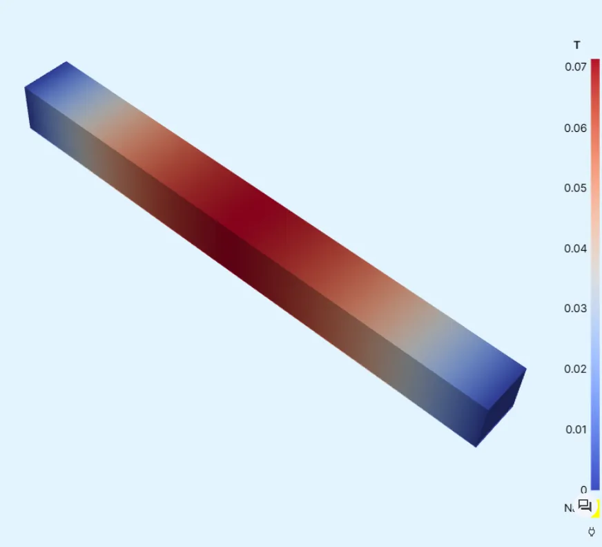
This simulation example focuses on AC Joule heating in a 1 mm length of aluminium wire, modeled as a simple rectangular piece. By simulating the flow of alternating current, we can visualize and quantify the heat distribution and temperature rise within the conductor.

Demo project: Harmonic balance - Joule heating AC

Simulation setup guide

Here you’ll find a simplified, example case level guide for setting up a aluminium wire AC joule heating simulation in Quanscient Allsolve.

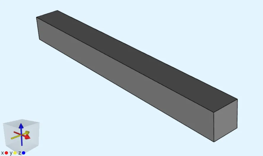
Step 1 - Build the geometry

In the Model section, build a box for the wire geometry:

Name	Element type	Center point [m]	Size [m]	Rotation [deg]
box	Box	X: 0	X: 1e-3	X: 0
		Y: 0	Y: 1e-4	Y: 0
		Z: 0	Z: 1e-4	Z: 0

Step 2 - Define shared expressions and materials

Go to the Properties section.

1. Define a shared expression:

   Name	Description	Expression
   freq	AC frequenzy [Hz]	5

2. Assign Aluminium to the wire volume.

   • Add the aluminium target as a shared region.

Step 3 - Define the physics

Go to the Physics section.

In this example, the Current flow and Heat solid physics are required. Add both of them before moving on to define interactions.

Physics 1 - Current flow

• Let current flow target default to the whole geometry.

• Add Constraint and name it as Ground:

  Name	Interaction type	Target	Value
  Ground	Constraint	End surface of beam in the negative X-direction (2)	0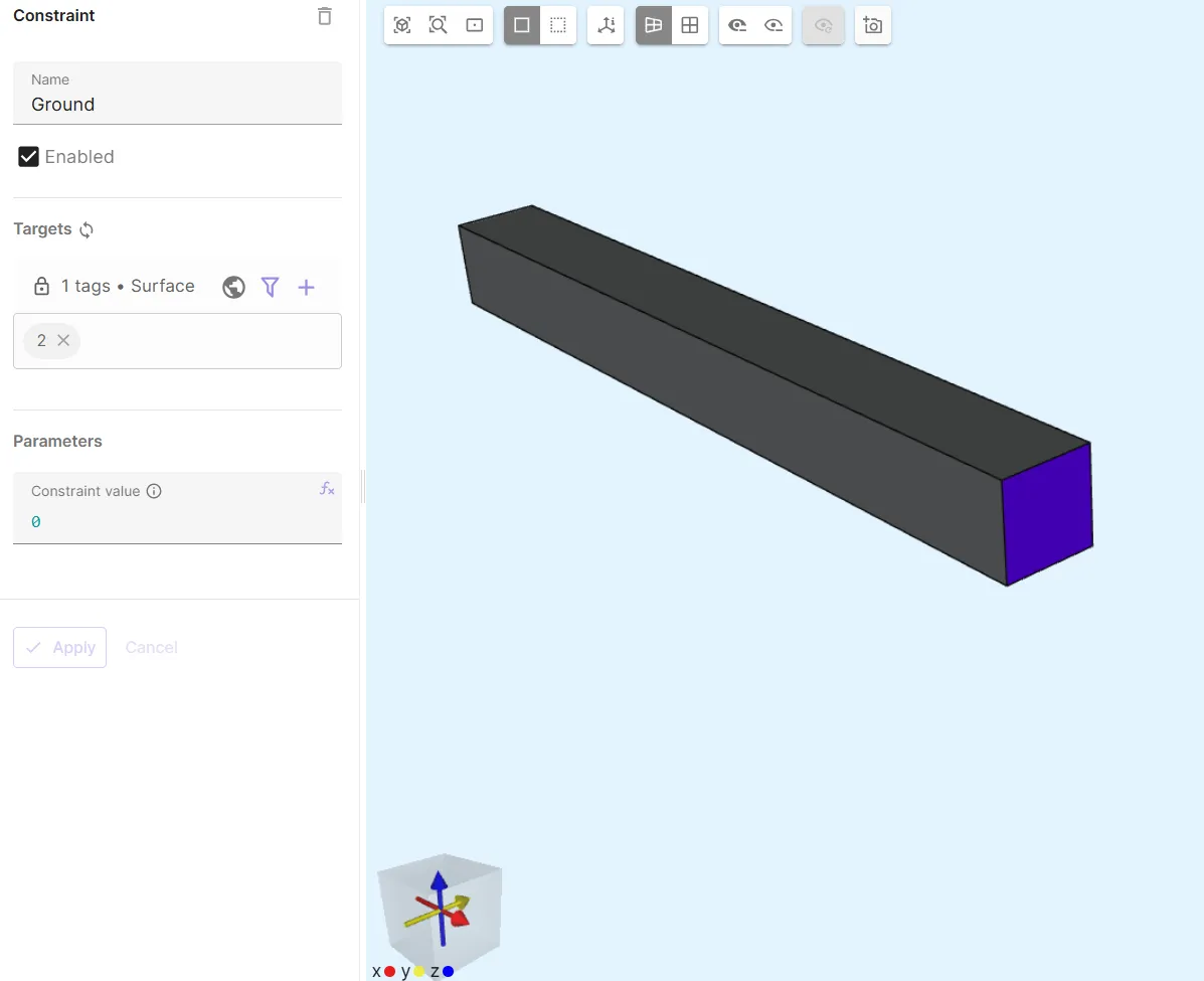

  

• Add Lump I/V:

  Name	Interaction type	Target	Actuation mode	Value
  Lump I/V	Lump I/V	End surface of beam in the positive X-direction (1)	Current	sn(1)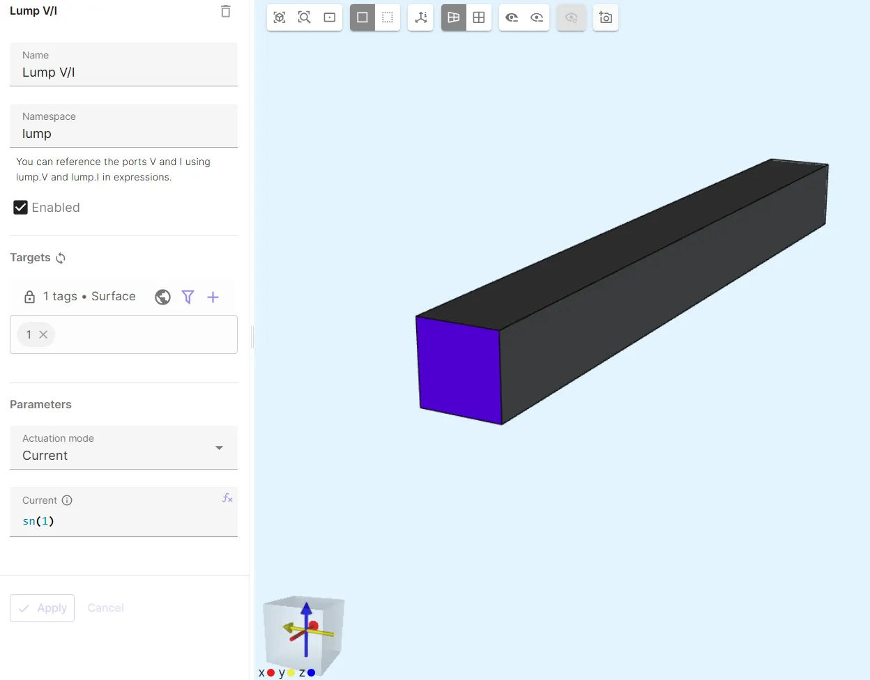

  

Physics 2 - Heat solid

• Let heat solid target default to the whole geometry.

• Add Constraint:

  Name	Interaction type	Target	Value
  Ground	Constraint	Both end surfaces of beam (1, 2)	0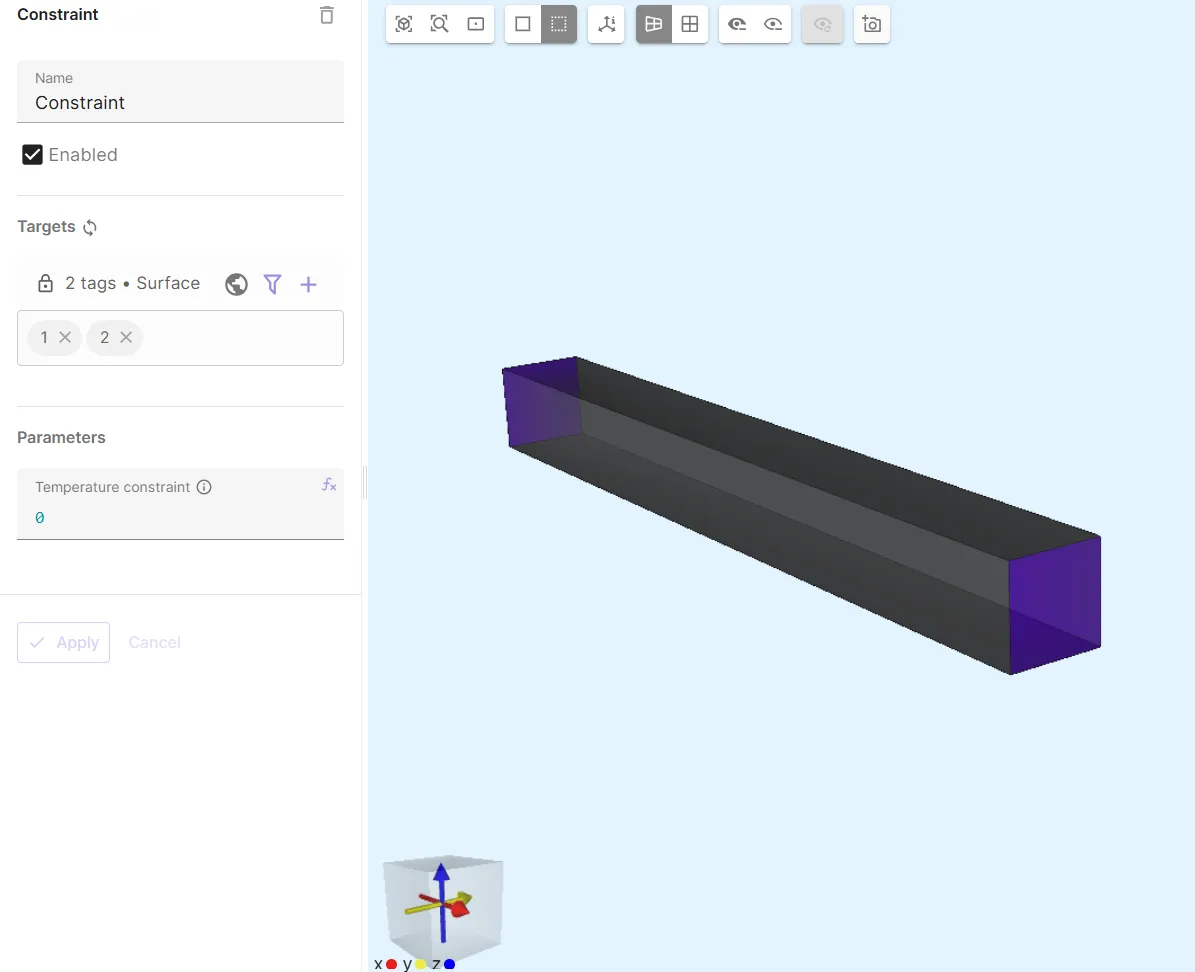

  

• Add Joule heating to couple Heat solid with Current flow.

  • As target, select the wire volume (1).

Step 4 - Generate the mesh

Go to the Simulations section.

Generate a mesh with default settings and check the preview.

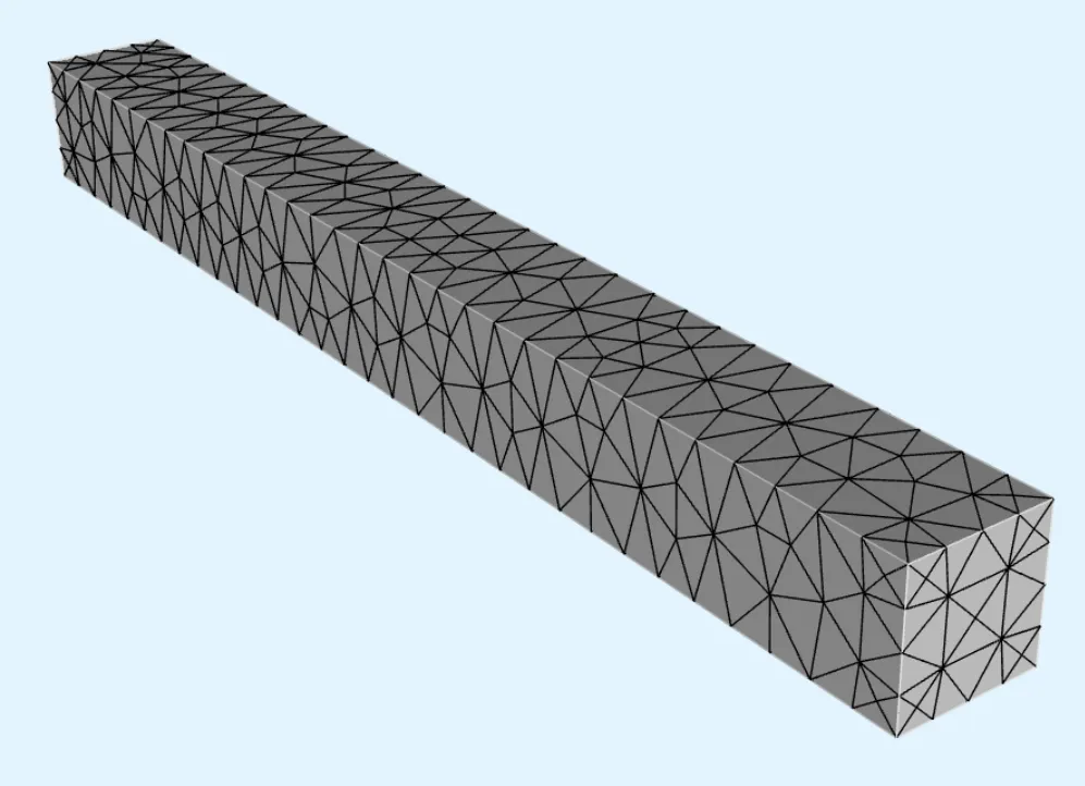
Step 5 - Simulate

Create a new simulation:

Analysis type	Fundamental frequency	Harmonics
Multiharmonic	freq	1, 2, 3, 4, 5

• As mesh, select the mesh you created.
• Inputs
  • Add freq sweep with override expression linspace(1, 501, 41).
• Outputs
  • Add custom value outputs:
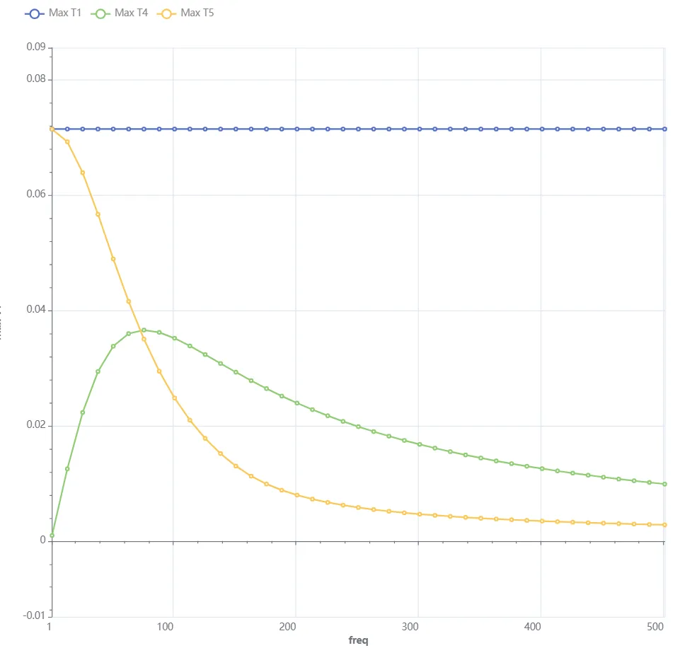
    • Max T1, output expression maxvalue(reg.aluminium_target, abs(harm(1, T)), 5)
    • Max T4, output expression maxvalue(reg.aluminium_target, abs(harm(4, T)), 5)
    • Max T5, output expression maxvalue(reg.aluminium_target, abs(harm(5, T)), 5)
  • Add Electric potential field v and Temperature field T outputs. All 5 harmonics are automatically added, but some give redundant results. Harmonics v1, v3, v4, v5 and T2, T3 can be removed, while keeping the following harmonics:
    • v harmonic 2
    • T harmonic 1
    • T harmonic 4
    • T harmonic 5
  • Harmonics v1, v3, v4, v5 as well as T2, T3 can be omitted as redundant.

You simulation is now ready to run.

Step 6 - Plot & visualize results

Add plots and visualizations to see results. Some examples are given below.

Max T outputs plotted

T harmonic 1 output visualized