MUTs 002 - Piezocomposite transducer
In this example case, a piezocomposite ultrasound transducer is simulated. Their main application is in medicine, where they are used for ultrasound imaging and medical therapeutics. Other applications include sonar and non-destructive testing.
The model captures a single element of a 1-3 piezocomposite linear array. The piezocomposite combines a soft PZT with an epoxy filler with a 40% volume fraction. The piezocomposite sits on a backing layer, and utilizes a 1/4 wavelength matching layer for better coupling into the water load. The centre element of the array is driven with a short voltage pulse to allow the wideband behaviour, or impulse response, of the device to be captured. Key outputs are:
- Drive voltage and current
- Pressure in the load
- Electrical impedance
Demo project: Piezocomposite demo V1
Simulation setup guide
Section titled “Simulation setup guide”Here you’ll find a simplified, example case level guide for setting up a piezocomposite transducer simulation in Quanscient Allsolve.
Step 1 - Define variables
Section titled “Step 1 - Define variables”Start out in the Common sidebar by defining variables:
| Name | Description | Expression |
|---|---|---|
| frequency | Frequency [Hz] | 1.25e6 |
| ncycles | Number of cycles | 5 |
| npillars | Number of pillars | 5 |
| thick_comp | Composite thickness [m] | 1e-3 |
| kerf | Cut width [m] | 0.15e-3 |
| pitch | Distance between cuts [m] | 0.4e-3 |
| pillar | Pillar width [m] | pitch-kerf |
| width | Element width [m] | npillars*pitch - kerf |
Step 2 - Build the geometry
Section titled “Step 2 - Build the geometry”-
Go the
Geometrysection. -
Start building the model geometry by adding Box elements:
Name Element type Center point [m] Size [m] Rotation [deg] pzt Box X: 0X: widthX: 0Y: 0Y: widthY: 0Z: thick_comp/2Z: thick_compZ: 0Name Element type Center point [m] Size [m] Rotation [deg] cut x Box X: 0X: widthX: 0Y: -width/2 + kerf/2 + pillarY: kerfY: 0Z: thick_comp/2Z: thick_compZ: 0Name Element type Center point [m] Size [m] Rotation [deg] cut y Box X: -width/2 + kerf/2 + pillarX: kerfX: 0Y: 0Y: widthY: 0Z: thick_comp/2Z: thick_compZ: 0 -
Use the Translate operation to copy the cuts in X and Y directions:
Name Element type Target Translation [m] Copy Repeat count copy x Translation cut y volume ( 25)X: pitchYes npillars - 2Y: 0Z: 0Name Element type Target Translation [m] Copy Repeat count copy y Translation cut x volume ( 13)X: 0Yes npillars - 2Y: pitchZ: 0 -
Use the Union operation to merge all the multiplied cuts to a single volume:
Name Element type Target combine polymer Union cut volumes ( 13, 25-31) -
Confirm model changes.
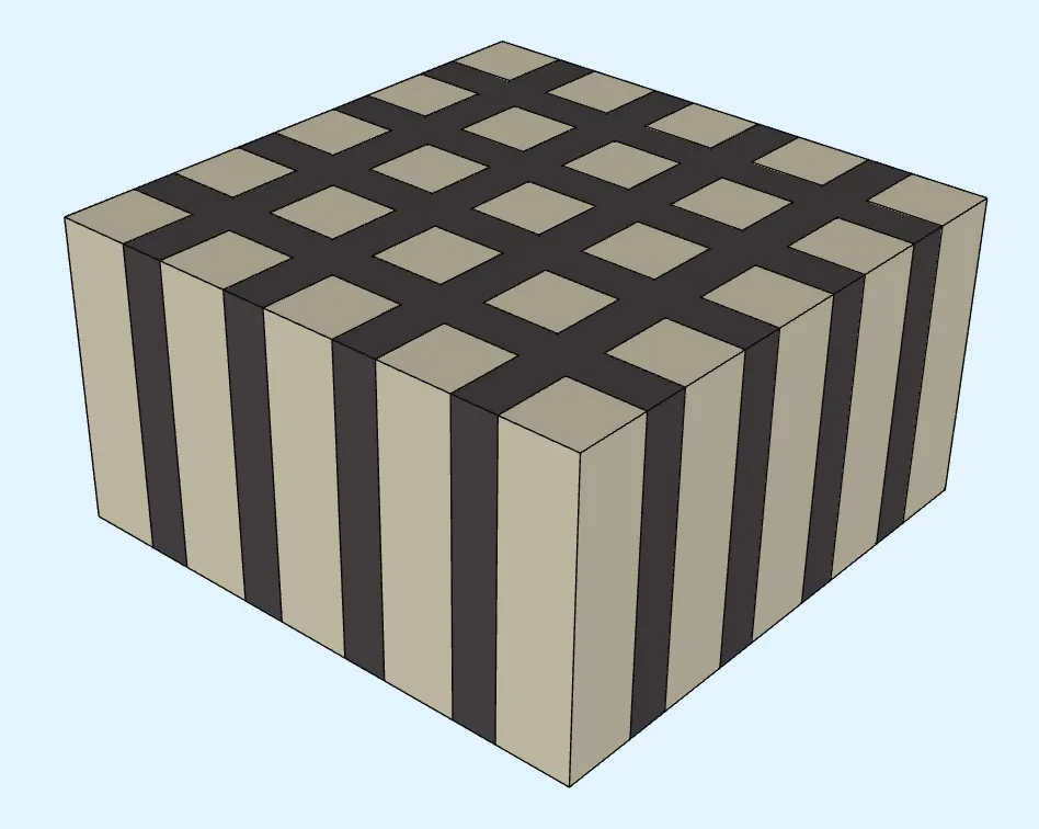
Finished geometry:
Step 3 - Define the materials
Section titled “Step 3 - Define the materials”Go to the Physics section to define model materials.
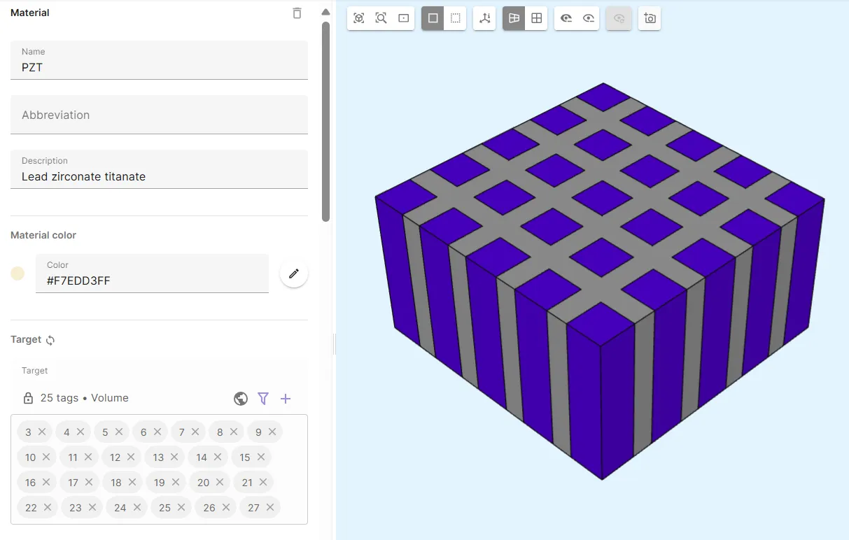
Material 1 - PZT
Section titled “Material 1 - PZT”Assign PZT to the piezoelectric pillars.
There are 25 of them in total. To save some clicks:
Select allvolumes- Remove the epoxy filler volume (
2) from your selection.
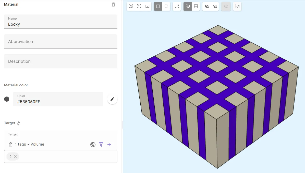
Material 2 - Epoxy
Section titled “Material 2 - Epoxy”Create a new material for the epoxy filler:
| Material | Target |
|---|---|
| Epoxy | Polymer filler volume (2) |
Define properties for Epoxy:
| Property | Value | Units |
|---|---|---|
| Density | 1134 | |
| Elasticity matrix | Poisson’s ratio: 0.37 | - |
Young’s modulus: 3.831e9 | ||
| Electric permittivity | 4*epsilon0 |
Step 4 - Define the physics
Section titled “Step 4 - Define the physics”Go to the Physics section.
The Elastic waves and Electrostatics physics are required for this example.
Add both of them before moving on to define interactions.
Physics 1 - Elastic waves
Section titled “Physics 1 - Elastic waves”- Let elastic waves target default to the whole geometry.
- Add the Elastic waves - Electrostatics coupling
Piezoelectricity.- Select the
PZT targetshared region as target.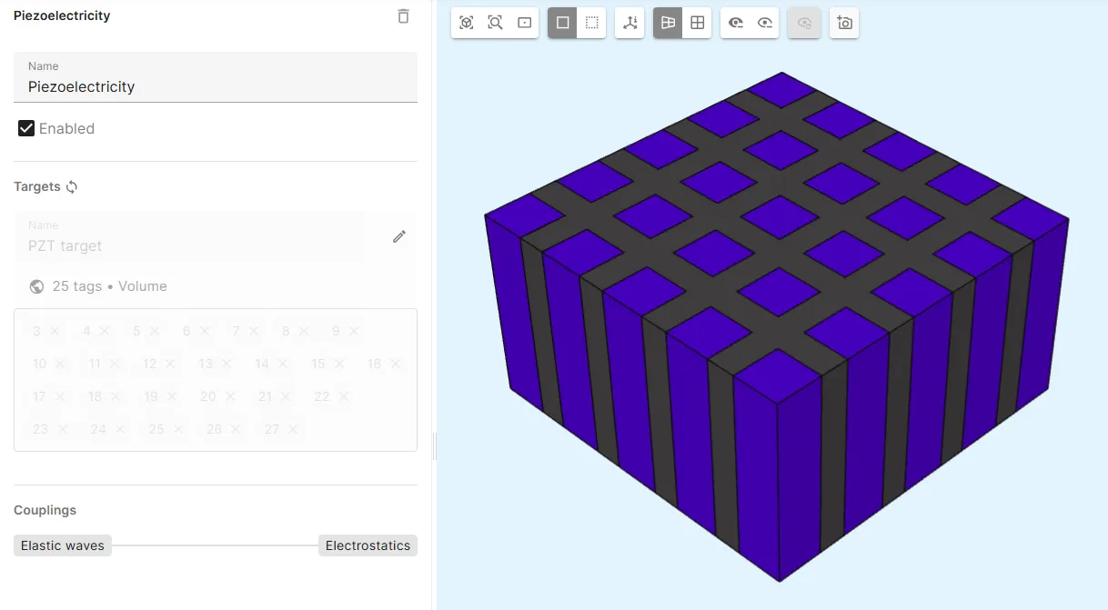
- Select the
Physics 2 - Electrostatics
Section titled “Physics 2 - Electrostatics”-
Let Electrostatics target default to the whole geometry.
-
Add a
Constraintinteraction which acts as a ground on the bottom surface:Interaction Target Constraint value ConstraintBottom surface of the element 0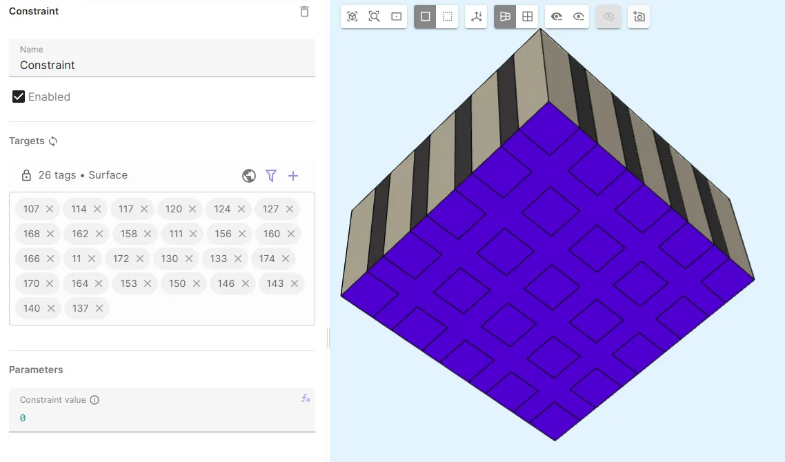
-
Add a
Lump V/Qinteraction which drives a voltage on the top surface:Interaction Target Voltage Lump V/QTop surface of the element wavelet(frequency, 1.2)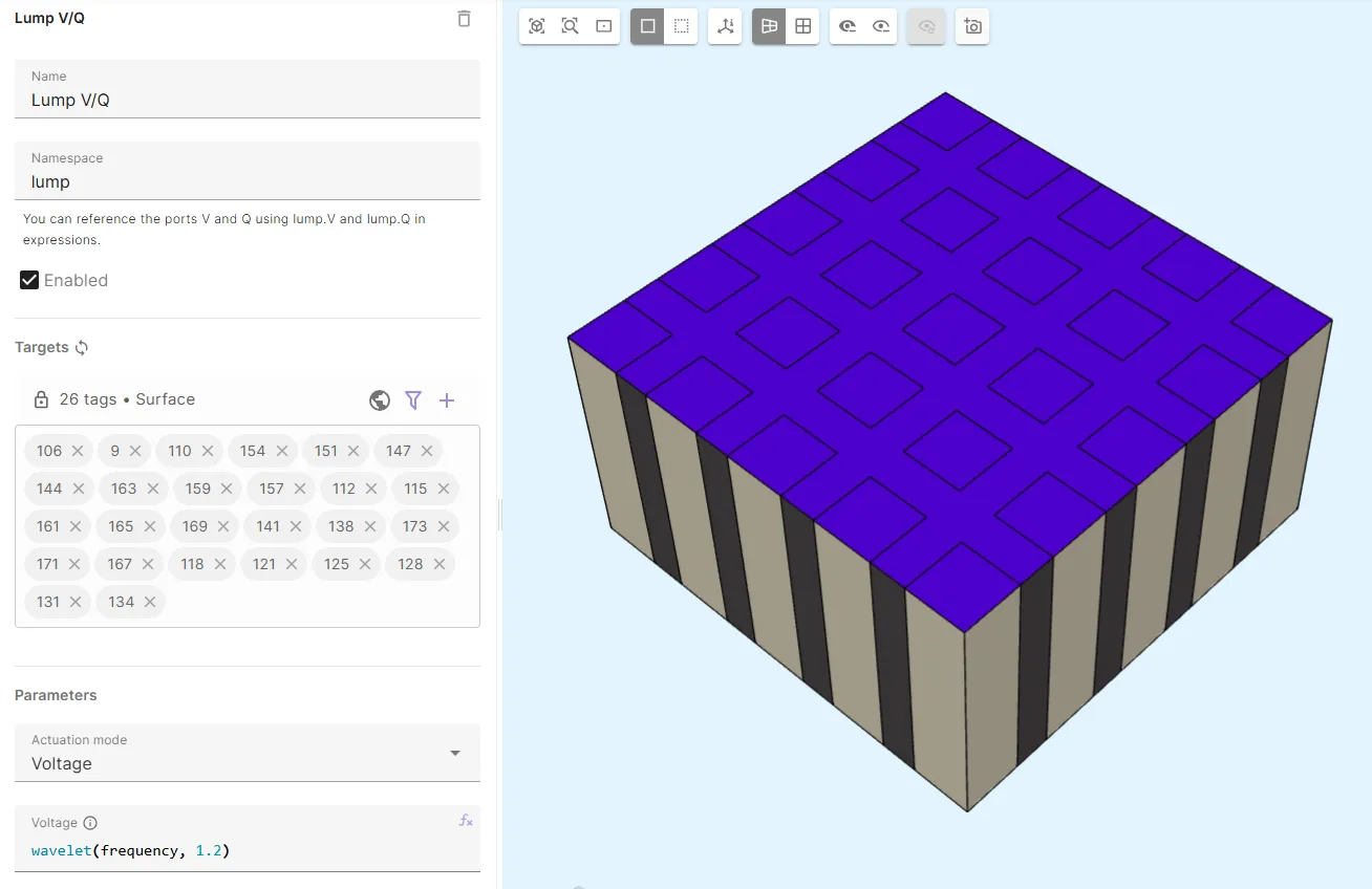
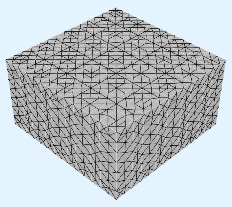
Step 5 - Generate the mesh
Section titled “Step 5 - Generate the mesh”Go to the Simulations section and create a new mesh:
- Set Mesh quality to
Expert settings. - Set Used mesher to
Basic. - Set Max size to
kerf. - Apply settings and mesh.
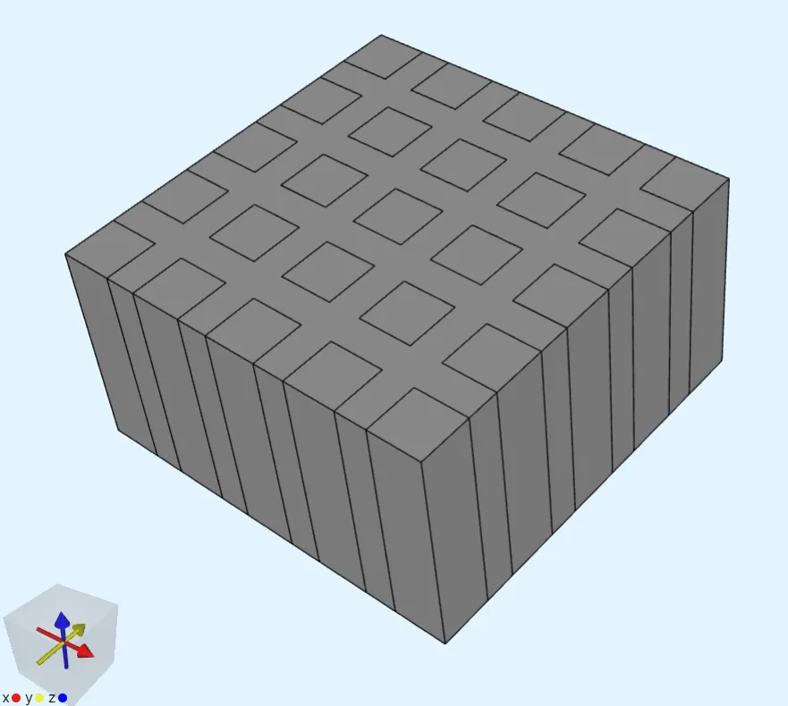
- Check the preview:
Step 6 - Simulate
Section titled “Step 6 - Simulate”In the Simulations section, create a new simulation:
-
Set Analysis type to
Transient. -
Select timestepping options:
Timestep algorithm Start time [s] End time [s] Timestep size [s] Generalized alpha0ncycles/frequency1/frequency/20 -
Select the mesh.
-
Add Outputs:
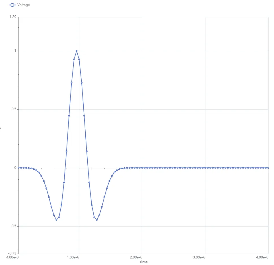
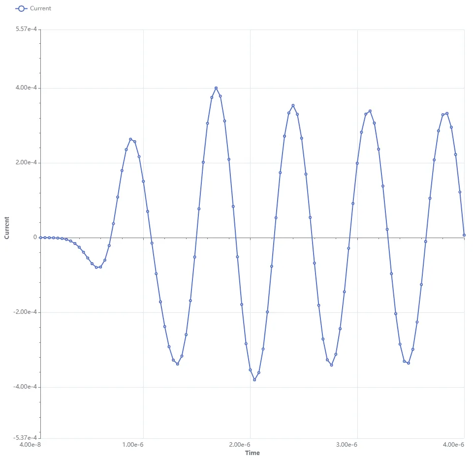
Output type Name Output expression Skin only Field Displacement field u uYes Custom value Voltage lump.VCustom value Current dt(lump.Q)
Your simulation is now ready to run.
Step 7 - Results
Section titled “Step 7 - Results”In the Simulations section, you can add plots to see value output results and visualizations to see field output results.
-
Voltage:
-
Current:
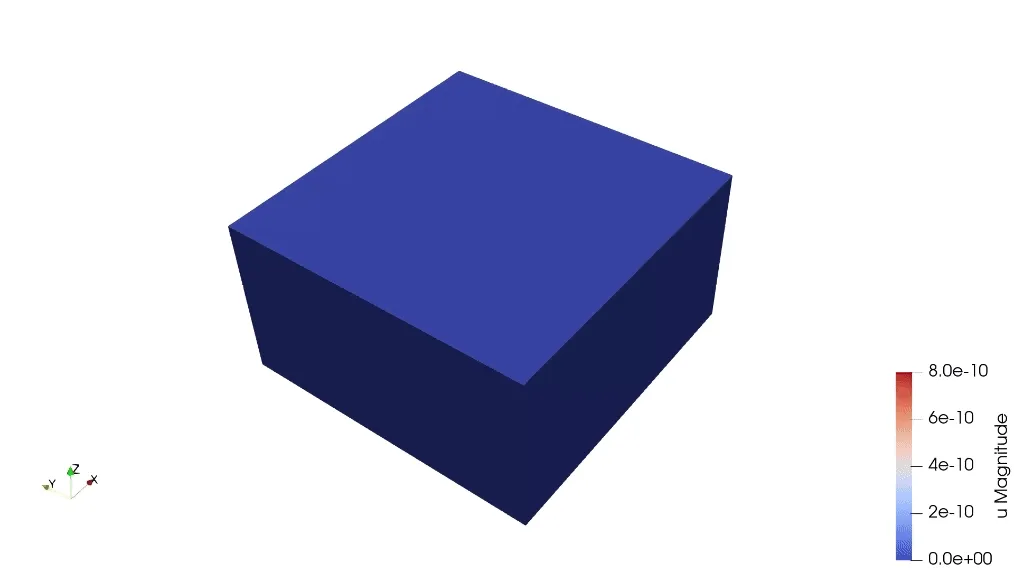
-
Displacement field: