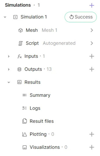
Results

Once a simulation has started running, Results can be accessed.

Under Results, there are 5 sections:

• Summary
  • See value outputs for each timestep or subsimulation.
• Logs
  • See simulation status messages.
• Result files
  • Download simulation results as .vtu or .json files.
• Plotting
  • Plot value outputs.
• Visualizations
  • Visualize field outputs.

Summary

In the Summary, you can keep track of all your value outputs. Value outputs are shown for each transient simulation timestep or sweep subsimulation.

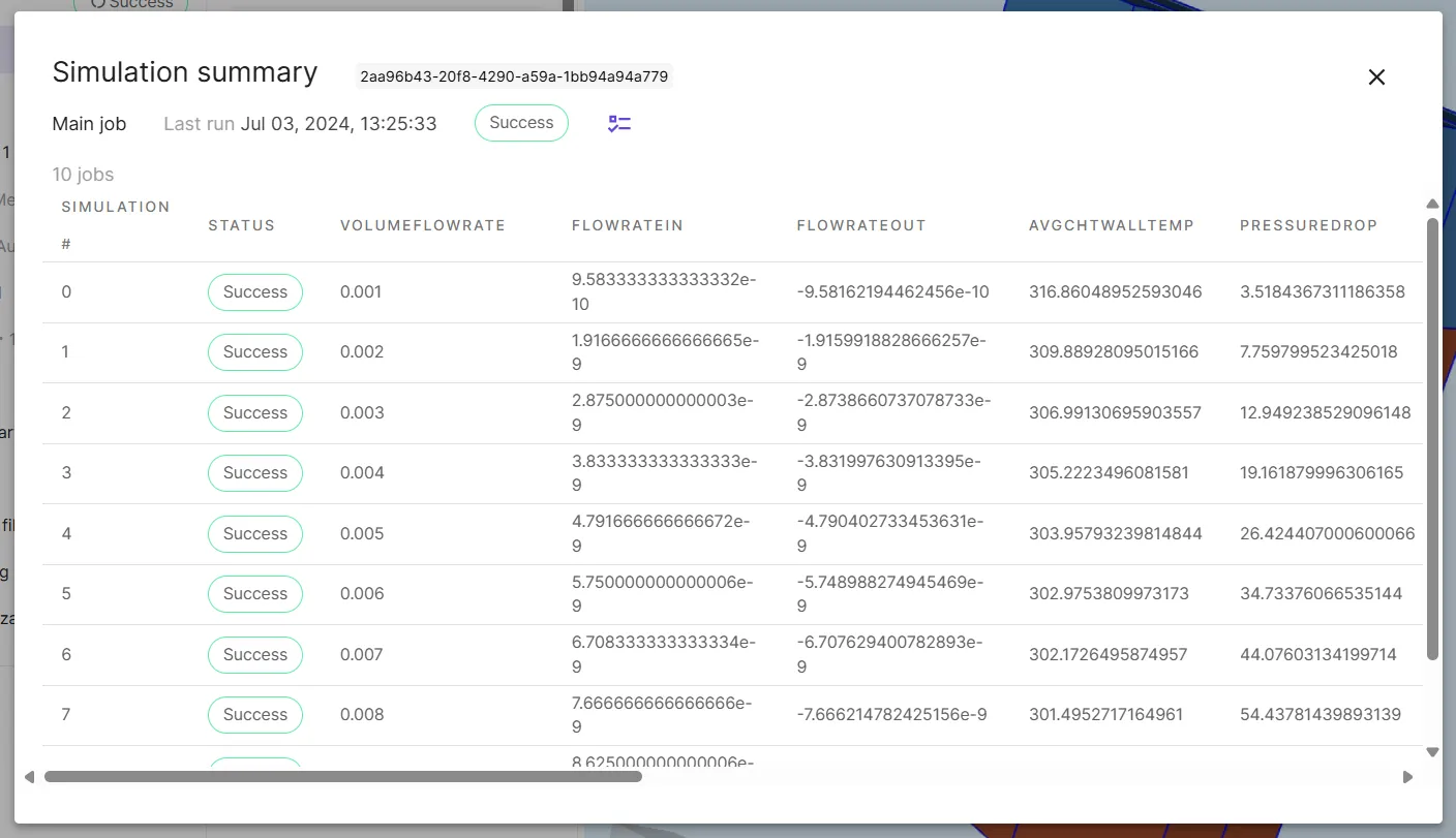
If an error occurs and a simulation run fails, you can check the summary status column to see at what point it occurred. Value outputs can also be exported as a .csv table from the summary.

Logs

Any status messages that are sent during simulation runs show up in the Logs. Taking a look at the simulation log is a good way to see what’s happening “under the hood” during simulation runs.

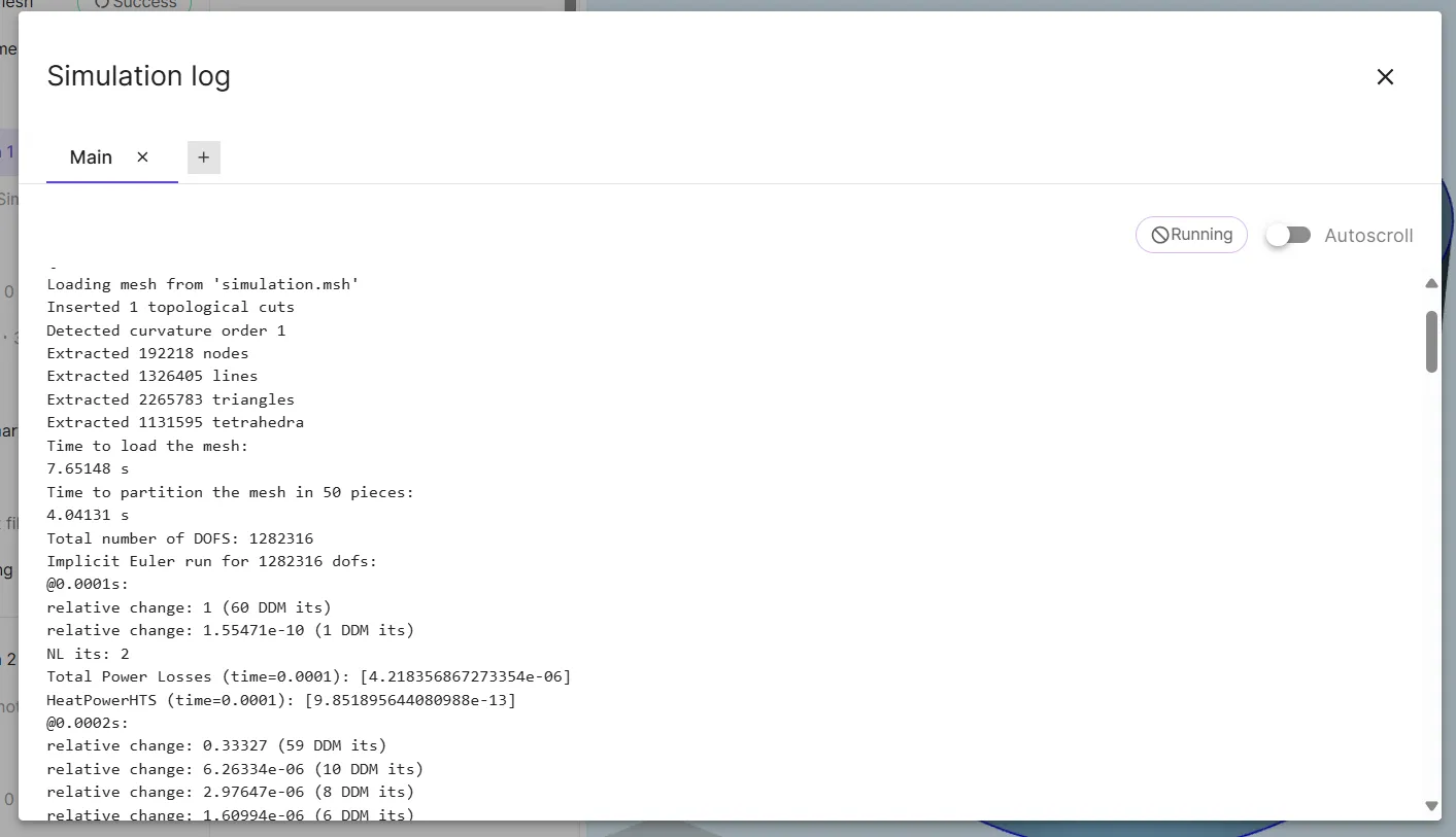
Any values can also be printed to the Logs by using the print function in script.

For a closer look at logs, see the dedicated page Simulation log.

Result files

In Result files, simulation results can be downloaded as .vtu or .json files.

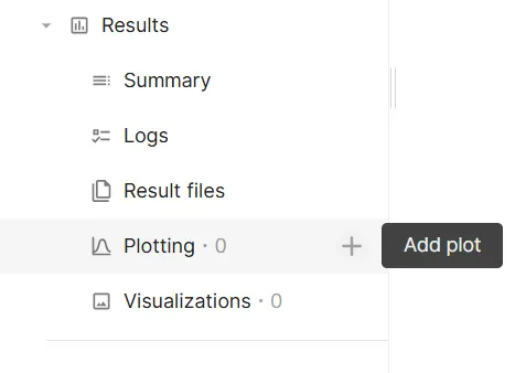
Plotting

In Plotting, simulation value outputs can be plotted.

To add a plot, click + next to Plotting:

Once a plot has been added, an automatic empty series is created but a single plot can have any number of different series.

Series options include:

• X value
  • Value to plot on the X-axis.
• Y value
  • Value to plot on the Y-axis.
• Series from
  • Optional.
  • Available when data dimensions exceed 2, for example in cases of transient sweep simulations.
  • Group data by a dimension, such as sweep step, and create series based on the groups automatically.
• Bound input
  • Optional.
  • Available when data dimensions exceed 3, for example in cases of transient sweep when plotting arrays values.
  • Bind a data dimension, such as array index, to be able to plot multidimensional data.

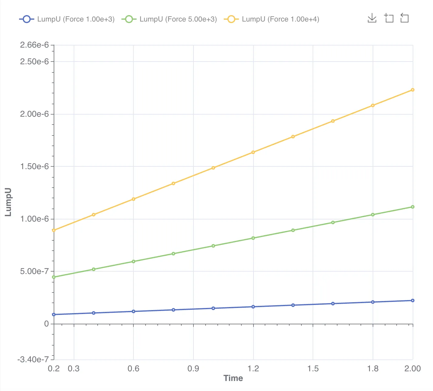
Example: Simple transient sweep

Let’s look at plotting the results of a simple transient sweep simulation for the bending of a cantilever beam. The simulation is setup as follows:

• The load Force * (1 + t) is applied in the negative Z-direction on the top surface of the beam.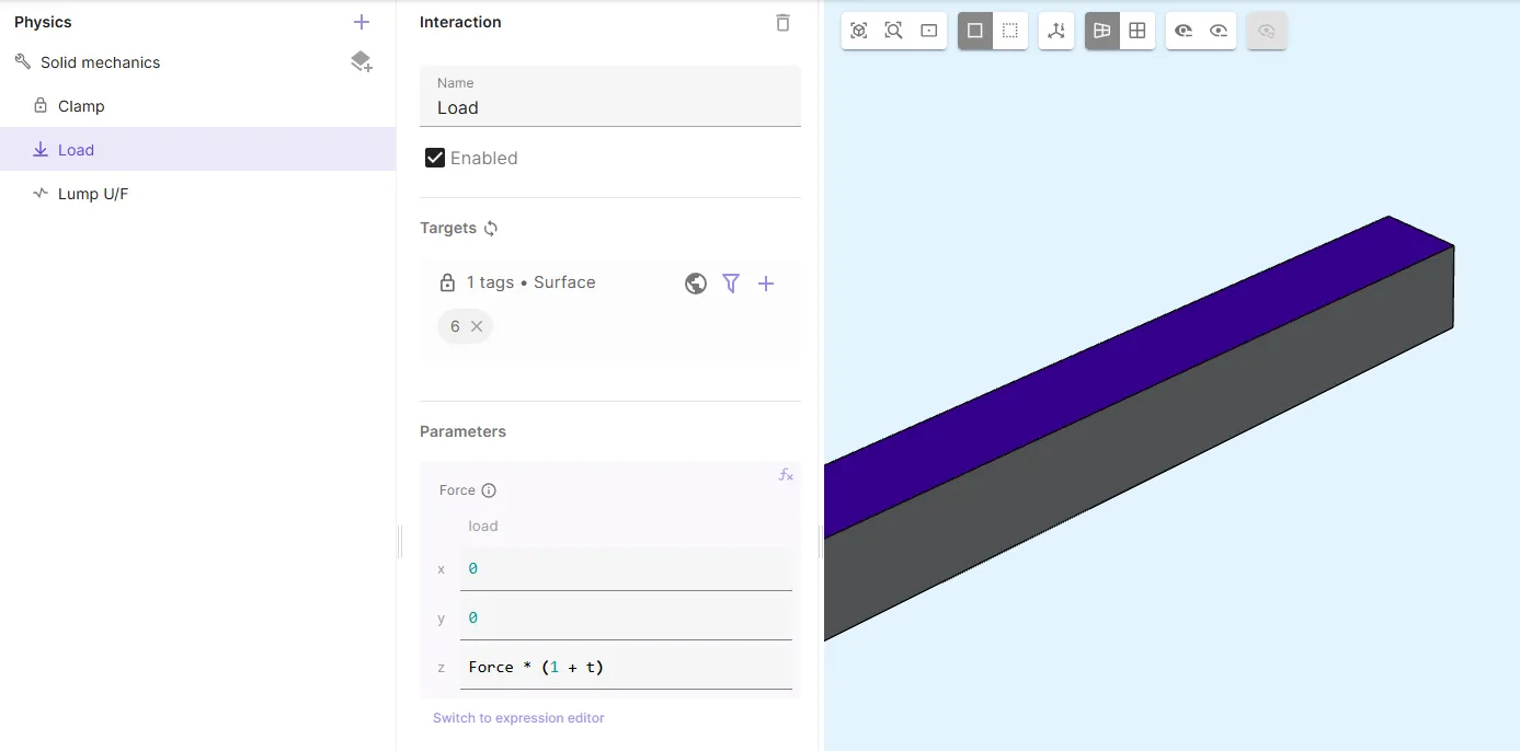
• The shared expression Force [N] is swept with 3 values, [1000, 5000, 10000].
• The transient simulation is run from 0 - 2 s with 0.5 s timesteps.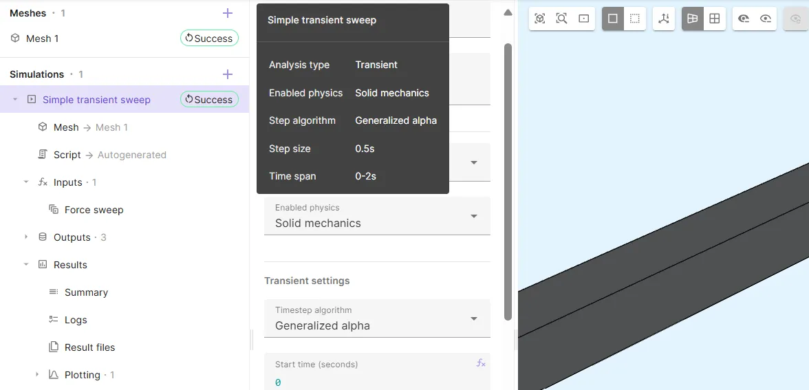

Plot options are chosen are chosen as follows:

• Time is plotted on the X-axis.
• The LumpU value output [lump.Ux, lump.Uy, lump.Uz] is plotted on the Y-axis.
• Force is selected as series grouping, so that separate series are formed for each sweep job and thus Force value.
• LumpU is a 3-valued array output ([lump.Ux, lump.Uy, lump.Uz]). Array index 2 is the Z-directional lumped displacement.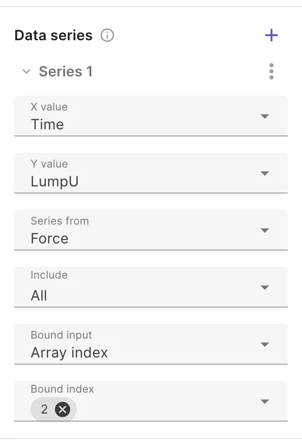

The plot automatically creates separate curves for each sweeped force value.

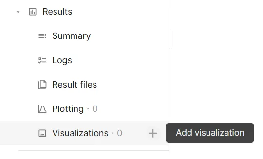
Visualizations

In Visualizations, field outputs can be visualized.

To add a visualization, click + next to Visualizations: