HB 002 - Backbone curve of a clamped-clamped beam

Beams are fundamental structural elements used in a wide range of applications, from bridges and aircraft to microelectronics. However, beams are susceptible to vibrations, which can lead to fatigue, instability, and potential failure. Therefore, understanding beam vibration behavior is essential for engineers across various disciplines.

This simulation example case investigates the multiharmonic vibration characteristics of a thin metal beam clamped at both ends. This “clamped-clamped beam” model provides insights into how boundary conditions influence vibrational behavior.

The model consists of a simple, thin beam made up of metal-like custom material. As simulation output, we take the maximum displacement of the beams harmonic displacement (vibration). When plotted, the displacement a so-called “backbone curve”. The setup is detailed in the paper Parallel harmonic balance method for analysis of nonlinear dynamical systems¹.

Demo project: ²(https://allsolve.quanscient.com/#/projects/428c622d-977f-4e82-a027-a51d5a489875)

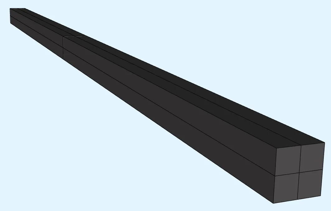
Step 1 - Build the geometry

Geometric entity tags

Geometric entities (volumes, surfaces, curves and points) are referenced using tags throughout this tutorial.

Carefully replicate the geometry construction steps below in order to have correct tags. Incorrect entity tags can lead to errors or unexpected behavior during simulations.

In the Model section, build boxes to make the beam geometry:

Name	Element type	Center point [m]	Size [m]	Rotation [deg]
Beam	Box	X: 0	X: 1	X: 0
		Y: 0	Y: 0.03	Y: 0
		Z: 0	Z: 0.03	Z: 0

Name	Element type	Center point [m]	Size [m]	Rotation [deg]
Beam half X	Box	X: 0.25	X: 0.5	X: 0
		Y: 0	Y: 0.03	Y: 0
		Z: 0	Z: 0.03	Z: 0

Name	Element type	Center point [m]	Size [m]	Rotation [deg]
Beam half Y	Box	X: 0	X: 1	X: 0
		Y: 0.0075	Y: 0.015	Y: 0
		Z: 0	Z: 0.03	Z: 0

Name	Element type	Center point [m]	Size [m]	Rotation [deg]
Beam half Z	Box	X: 0	X: 1	X: 0
		Y: 0	Y: 0.03	Y: 0
		Z: 0.0075	Z: 0.015	Z: 0

Copying elements

The elements in this geometry have many identical values, so it’s a good idea to copy each new box from the last:

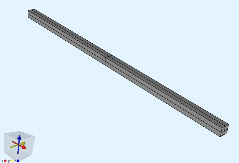
Finished geometry:

Confirm model changes before moving on.

Step 2 - Define variables and materials

Go to the Common sidebar.

1. Define a variable:

Name	Description	Expression
freq	Fundamental frequency for multiharmonic simulation [Hz]	162.5

Go to Physics section

2. Create a custom material for the beam:

Name

• Material from paper

Material name

Make sure to name the material Material from paper.

It is later referred to in an output definition by that name, and the reference will not work otherwise.

Target

• All volumes 1-8
  • Add the target as a shared region.

Properties

• Add Density
  • Set value to 7800 [kg / m^3]
• Add Elasticity matrix
  • Set Poisson’s ratio to 0.3
  • Set Young’s modulus to 210e9 [Pa]

Step 3 - Define the physics

For this example, only Solid mechanics is required. Add it and define interactions:

• Let solid mechanics target default to all volumes.
• Add Clamp.
  • As target, select end surfaces of the beam in positive and negative X-planes (1, 7, 12, 19, 22, 29, 33, 36).
• Add Load and name it as Center point load.

Load interaction name

Make sure to name the load physics as Center point load. It is later referenced by that name in scripting.

• As target, select the middle-most point of the beam inside the volume (7).
• Set Force to [0; 0; -200*sn(1)].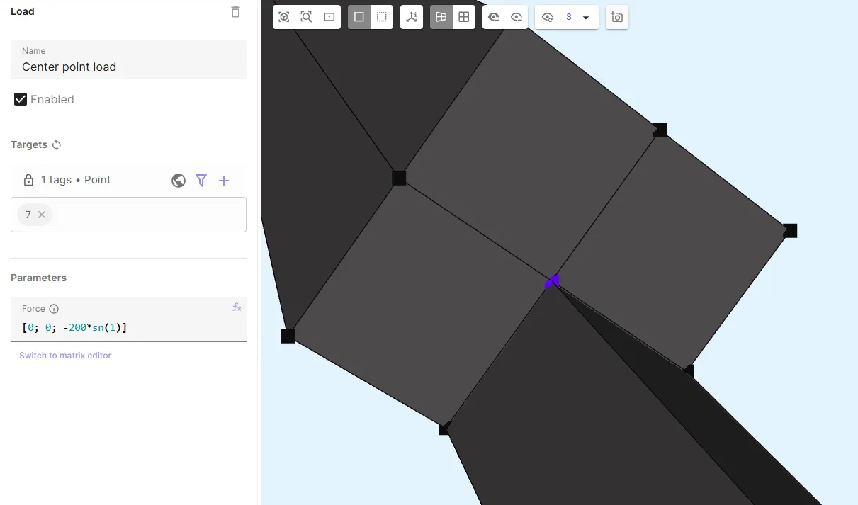
• Add Geometric nonlinearity.
• Add Proportional damping to all volumes. Use Rayleigh mass damping only, with Alpha = 3. Neglect stiffness-proportional damping by setting Beta = 0.

Step 4 - Generate the mesh

Go to the Simulations section. In this example, the geometry is meshed via Transfinite meshing.

1. Create a new mesh.
   • Set Mesh quality to Expert settings.
   • Set Used mesher to Basic.
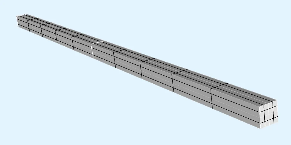
2. Create a transfinite entity for each of the 8 volumes in the model.
3. Before defining segment counts for the entities, apply mesh settings to save your work so far.
4. For each transfinite entity, choose segment counts so that the long sides are divided into 5 segments, and the short sides into 2 segments.
5. Apply settings and mesh.

Caution: Segment identifiers

The curve identifiers A/B/C may differ between volumes, so be careful to pick correct segment counts for each volume.

Step 5 - Simulate

In the Simulations section, create a new simulation:

• Analysis type

  • Multiharmonic

• Fundamental frequency

  • freq

• Harmonics

  • 1, 2, 3

• Solver mode

  • Direct solver

• Mesh

  • Select the mesh you created in Step 4.

• Scripting

  • The backbone curve can be computed using either the u-strategy or the f-strategy. Replace your script with the version below, which applies the u-strategy.

var = Variables()
mesh = Mesh()
fld = Fields()

# Load the mesh
mesh.mesh = qs.mesh()
mesh.mesh.setphysicalregions(*reg.get_region_data())
mesh.skin = reg.get_next_free()
mesh.mesh.selectskin(mesh.skin)
mesh.mesh.partition()
mesh.mesh.load("gmsh:simulation.msh", mesh.skin, 1, 1)

# Displacement field
fld.u = qs.field("h1xyz", [1, 2, 3])
fld.u.setorder(reg.all, 2)

# Clamp interaction
fld.u.setconstraint(reg.clamp_target)

maxuf2 = qs.sqrt(fld.u.harmonic(2)*fld.u.harmonic(2) + fld.u.harmonic(3)*fld.u.harmonic(3))

# Driving frequency loop with field solution from previous iteration as initial guess:
freqmin = 158.0
freqmax = 178.0
freq = freqmax
dir = -1
step = 0.25
arcindex = 0
nfft = 6

while True:

    qs.printonrank(0, "Solving for frequency " + str(freq) + " with direction " + str(dir))

    qs.setfundamentalfrequency(freq)

    form = qs.formulation()

    # Solid mechanics
    form += qs.integral(reg.all, nfft, qs.predefinedelasticity(qs.dof(fld.u), qs.tf(fld.u), fld.u, par.H(), 0.0))
    # Inertia terms
    form += qs.integral(reg.all, nfft, -par.rho() * qs.dtdt(qs.dof(fld.u)) * qs.tf(fld.u))

    # Load interaction: Center point load
    form += qs.integral(reg.center_point_load_target, nfft, qs.array3x1(0.0, 0.0, -200.0 * qs.sn(1)) * qs.tf(fld.u))

    # Rayleigh mass damping only: C = alpha * M
    alpha = 3.0
    form += qs.integral(reg.all, -alpha * par.rho() * qs.dt(qs.dof(fld.u)) * qs.tf(fld.u))

    # Continuation logic:
    isrisingbutnottoomuch = False
    umaxprev = qs.allmax(reg.material_from_paper_target, maxuf2, 2)
    ubkp = qs.vec(form)
    ubkp.setdata()
    nlindex = 0
    maxnlits = 10
    while nlindex < 5:
        numnlits = form.allsolve(relrestol=1e-06, maxnumit=1000, nltol=1e-05, maxnumnlit=maxnlits, relaxvalue=-1)
        curumax = qs.allmax(reg.material_from_paper_target, maxuf2, 2)
        if curumax > umaxprev and (umaxprev == 0 or curumax < 1.5*umaxprev) and numnlits < maxnlits:
            isrisingbutnottoomuch = True
            break
        qs.printonrank(0, "Not rising - Retrying: umaxprev was " + str(umaxprev) + " umax is " + str(curumax))
        # Reset and raise the guess for the next attempt:
        nlindex = nlindex+1
        qs.setdata((1.0+nlindex*0.05)*ubkp)

    # Value output: Max u f2
    var.discrete = qs.allmax(reg.material_from_paper_target, maxuf2, 2)

    if isrisingbutnottoomuch:
        qs.setoutputvalue("Frequency", freq, freq)
        qs.setoutputvalue("Max u f2 - arc "+str(arcindex), var.discrete, freq)
    else:
        dir = -dir
        arcindex = arcindex + 1
        if arcindex == 2:
            freq = freqmin
            dir = 1
            fld.u.setvalue(reg.all)
        if arcindex == 4:
            break

    freq = freq + dir*step

Your simulation is now ready to run!

Step 6 - Plot results

In the Simulations section, add three plots called Max u f2 - arc 0, Max u f2 - arc 1, and Max u f2 - arc 2 as a function of frequency. The results should resemble this:

In the Simulations section, add three plots named Max u f2 – arc 0, Max u f2 – arc 1, and Max u f2 – arc 2, each showing the maximum displacement. Plot the result as a function of Frequency. The results should look similar to the example below:

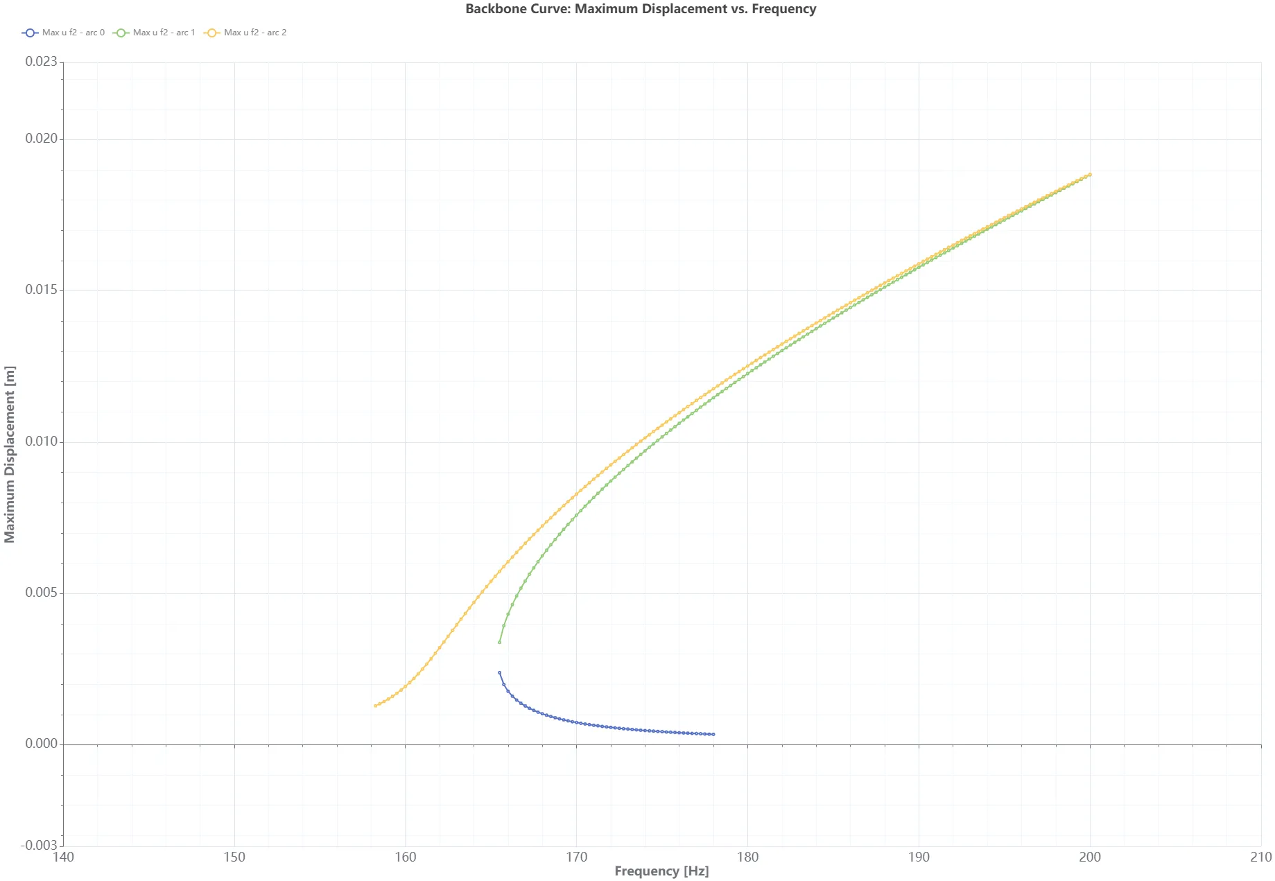
The figure illustrates the backbone curve bending towards higher frequencies.

Linear case

In a linear case, the resonance peak remains centered at a fixed frequency, producing a vertical straight peak as shown in the example below.

References

Footnotes

1. Paper: Parallel harmonic balance method for analysis of nonlinear dynamical systems https://asmedigitalcollection.asme.org/GT/proceedings/GT2020/84232/V011T30A028/1095387 ↩

2. Demo project: Backbone curve of a clamped-clamped beam https://allsolve.quanscient.com/#/projects/428c622d-977f-4e82-a027-a51d5a489875 ↩