MEMS 001 - Combdrive eigenmodes
In this example case, eigenmode analysis is done for a MEMS comb-drive accelerometer.
Model definition
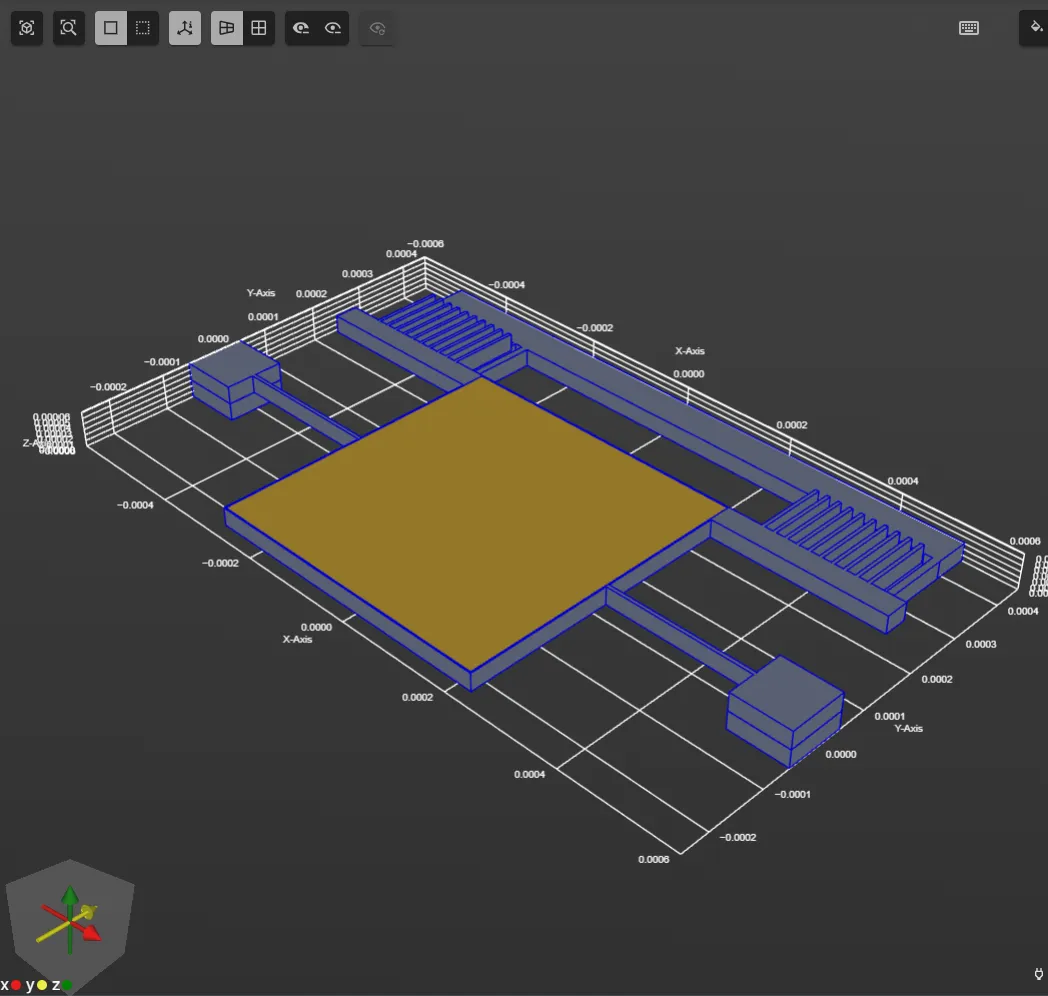
Section titled “Model definition”The comb-drive CAD model is illustrated below:
Simulation setup guide
Section titled “Simulation setup guide”Here, you’ll find a simplified guide on setting up this simulation in Quanscient Allsolve.
Step 1 - Create the geometry
Section titled “Step 1 - Create the geometry”-
In the
Geometrysection, start by importing a.gdsfile for the model.File download link: Comb-drive_Accelerometer.gds.
-
After importing, Allsolve recognizes 6 layers in the model. Perform the layer stackup:
-
Add 5 of the 6 suggested layers in this order:
11, 1, 12, 2, 23. -
Enter layer thicknesses:
Layer id Layer thickness [μm] Layer Z-position 23 0.1061.252 30.0031.2512 0.25311 30.00111 1.000Check that layer order and Z-positions match.
-
The excluded layer
63is a substrate on which the MEMS device is fixed. In this simulation, the substrate is replicated by clamping the bottom-most surfaces of the device. Hence, the substrate layer can be safely excluded from the geometry.
-
Step 2 - Define the materials
Section titled “Step 2 - Define the materials”Proceed to the Physics section to define the model materials.
Pick the Gold material from the materials library and assign it to volume 10. Click Apply.
Next, pick the Silicon dioxide material from the materials database. As the target, select volumes 1, 2, 3, 7 and 8. Click Apply.
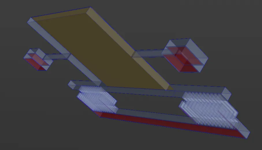
Finally, pick the Monocrystalline silicon material from the materials database. As the target, select volumes 4, 5, 6 and 9. Click Apply.
At this point, your model should look like in the image below (Translucent model with Silicon dioxide volumes highlighted in red).
Step 3 - Define the physics
Section titled “Step 3 - Define the physics”Proceed to the Physics section to define the physics.
For eigenmode analysis, Solid mechanics is the only physics required. Under Solid mechanics, add Clamp. As the clamp target, select volumes 1, 2 and 3. Click Apply.
Step 4 - Set up the mesh
Section titled “Step 4 - Set up the mesh”Proceed to the Simulations section to set up the mesh:
- Create a new mesh with
Mesh qualityset toExpert settings. - Set Used mesher as
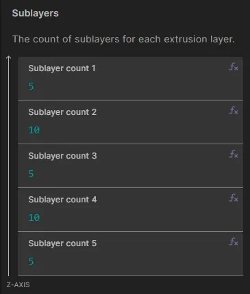
Basicand scale factor as0.25. - Scroll down and click
+next to Mesh extrusion. Pick the simple extrusion. As target volume, clickSelect allto select all volumes. Now, the mesh extrusion tool should recognize five separate layers. - Set the sublayer counts as in the image below.
- Click
Apply & mesh.
Step 5 - Simulate
Section titled “Step 5 - Simulate”In the Simulations section, create a new simulation with the following options:
- Set Analysis type as
Eigenmode. - Set Number of requested modes as
5. - Set Target eigenfrequency as
0. - Set Solver mode as
Iterative solverand set Relative residual tolerance as1e-6. - As the Mesh, select the mesh you just created.
- Next to Output, click
+and addDisplacement field uas a Field output.- Let the
ufield target default to the whole geometry. - Under Parameters, enable
Skin only. This should drastically reduce visualization loading times.
- Let the
Run the simulation by clicking Not Run.
Step 6 - Visualize
Section titled “Step 6 - Visualize”In the Simulations section, add a visualization to see u field results:
- Under Results, next to Visualizations, click
+. - On the visualization, add
u (real)andWarp. - Set the warp
Scale factorto1e-3. - Click
Apply.
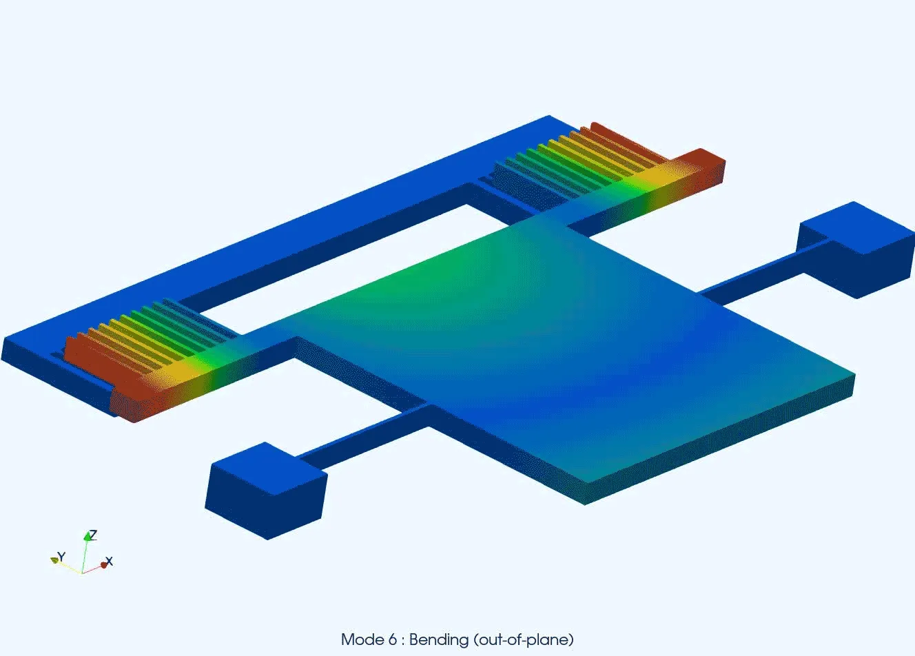
You can step through the different eigenmodes in the top-right corner of Model view. Below is eigenmode 6 post-processed as a gif.