CHT 002 - 2D Taylor-Couette flow
In this example, conjugate heat transfer (CHT) in a quasi-2D Taylor-Couette flow is simulated.
Taylor-Couette flow, characterized by the rotation of concentric cylinders and the fascinating patterns that emerge within the fluid, exhibits diverse flow regimes depending on the rotation speeds and fluid properties.
While traditional Taylor-Couette studies often focus on fluid mechanics, incorporating heat transfer adds another layer of complexity and practical relevance. In many real-world scenarios, the rotating cylinders and the fluid have different temperatures, leading to heat exchange between them. This is where CHT simulation becomes essential.
Model definition
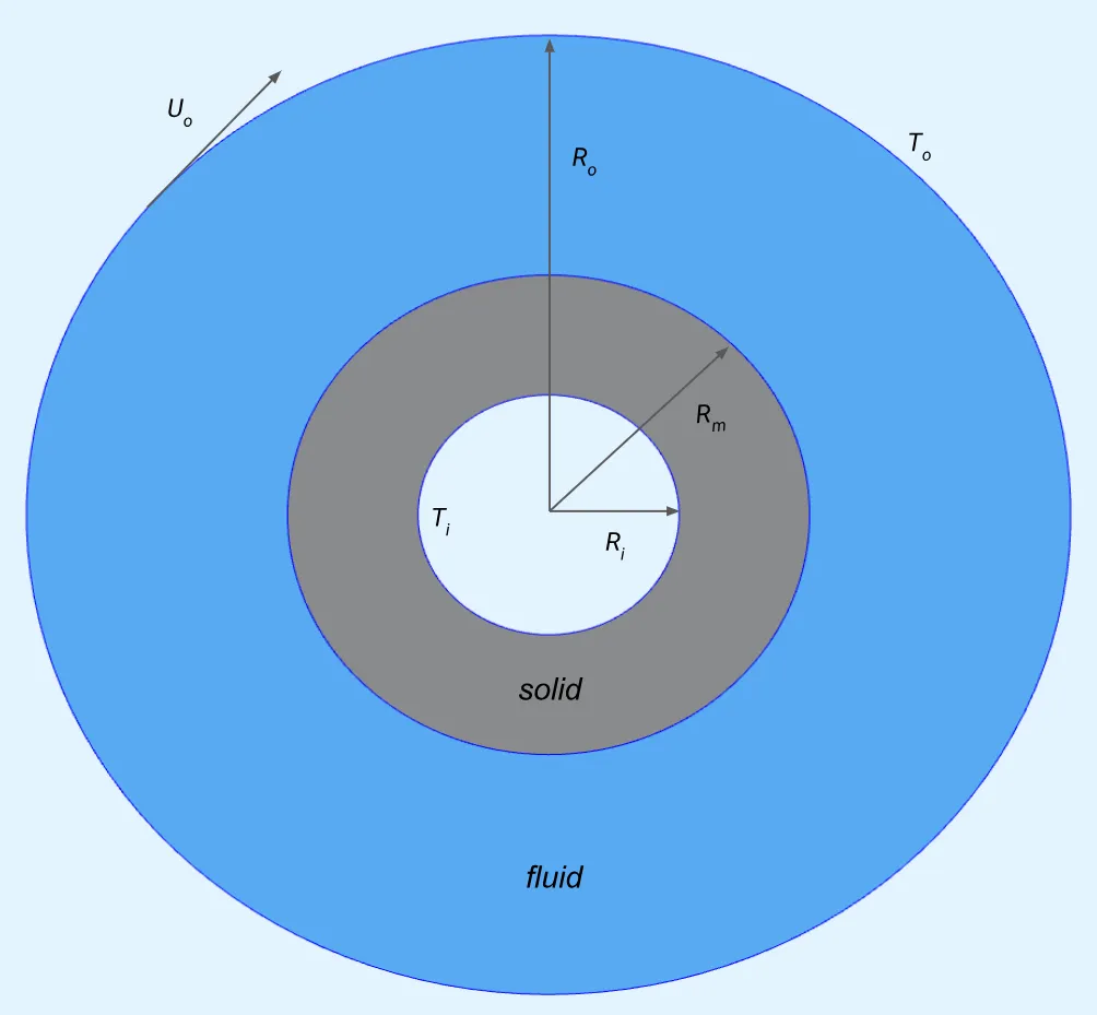
Section titled “Model definition”The model is composed of a thin disc with two hollow concentric cylinders: the inner hollow cylinder forms a solid region and the outer hollow cylinder forms the fluid region.
Demo project: Conjugate heat transfer
The model setup is based on a paper by De Marinis et al. 1
- The outer surface (at radius ) of the outer cylinder is rotating with a tangential velocity .
- The temperature at the outer surface is fixed at .
- The inner cylinder is stationary.
- The temperature at the inner surface of the inner cylinder is fixed at .
- At the interface of the solid and fluid region (surface at ), a no-slip velocity constraint is applied.
For Taylor-Couette flow, typically a viscous fluid is considered. Typical water properties are used for the fluid here, but kinematic viscosity is increased to to make it viscous. Normally, water has a kinematic viscosity of .
For the simulation setup in Allsolve, the tangential velocity is split into its X and Y components as detailed below. The heat transfer at fluid-solid interface is strongly coupled, therefore, no additional flux boundary conditions are required at the interface.

Simulation setup guide
Section titled “Simulation setup guide”Here you’ll find a simplified, example case level guide for setting up a conjugate heat transfer simulation in a quasi-2D Taylor-Couette flowing cylinder in Quanscient Allsolve.
Step 1 - Define variables
Section titled “Step 1 - Define variables”Start out in the Common sidebar by defining the following variables:
| Name | Description | Expression |
|---|---|---|
| Ro | outer radius [m] | 1.8 |
| Rm | interface radius [m] | 0.9 |
| Ri | inner radius [m] | 0.45 |
| h | height [m] | 0.05 |
| To | temperature at Ro [K] | 700 |
| Ti | temperature at Ri [K] | 500 |
| Uo | tangential velocity at Ro [m/s] | 2.0 |
| w | angular velocity at Ro [rad/s] | Uo/Ro |
| ksbykf | heat conductivity ratio between solid and fluid | 9.0 |
| nu | kinematic viscosity of fluid [m²/s] | 1.0 |
Step 2 - Build the geometry
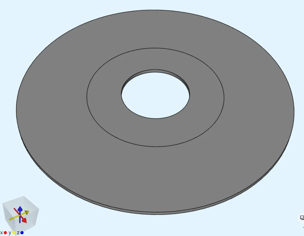
Section titled “Step 2 - Build the geometry”In the Model section, build the model geometry by creating Cylinders and by using the Fragment all and Remove operations as follows.
-
Create 3 cylinders:
Name Element type Center point [m] Size [m] Rotation [deg] inner cylinder Cylinder X: 0Radius: RiX: 90Y: 0Height: hY: 0Z: 0Z: 0Name Element type Center point [m] Size [m] Rotation [deg] interface cylinder Cylinder X: 0Radius: RmX: 90Y: 0Height: hY: 0Z: 0Z: 0Name Element type Center point [m] Size [m] Rotation [deg] outer cylinder Cylinder X: 0Radius: RoX: 90Y: 0Height: hY: 0Z: 0Z: 0 -
Apply the
fragment alloperation. -
Apply the
removeoperation, with the innermost small cylinder (volume1) as target.
Finished geometry:
Step 3 - Define the materials
Section titled “Step 3 - Define the materials”Go to the Physics section to define the model materials.
Material 1 - Water
Section titled “Material 1 - Water”Assign Water to the outer cylinder (volume 3).
Add the target as a shared region.
- Set the Dynamic viscosity of water to
par.rho()*nu.
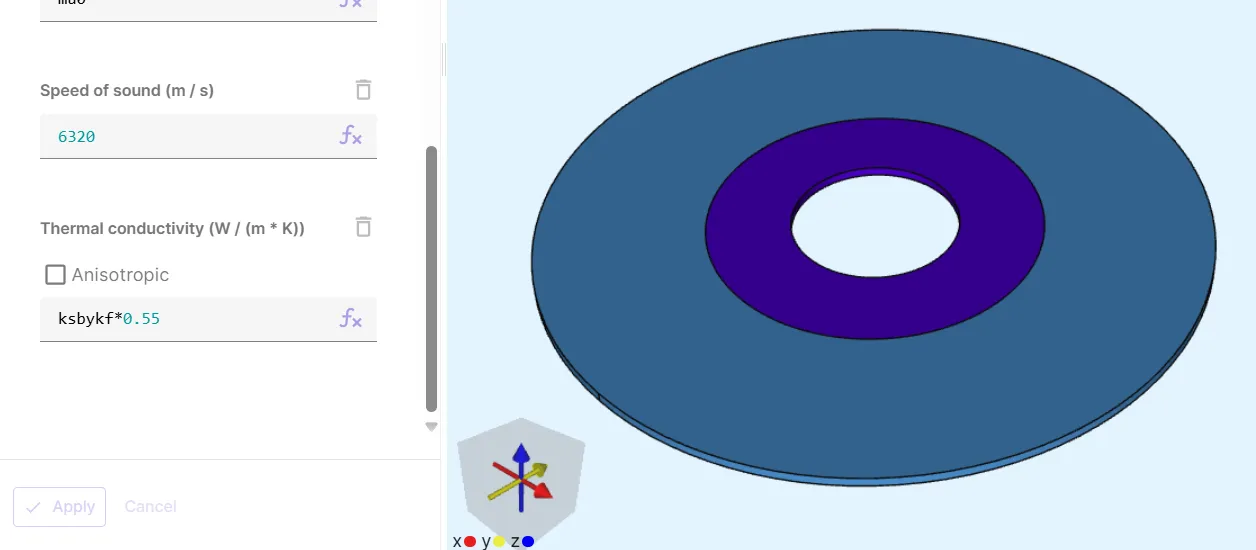
Material 2 - Aluminium
Section titled “Material 2 - Aluminium”Assign Aluminium to the interface cylinder (volume 2).
Add the target as a shared region.
- Set the Thermal conductivity of aluminium to
ksbykf*0.55.- Here,
0.55is the thermal conductivity of water.
- Here,
Your model materials are now defined.
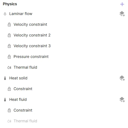
Step 4 - Define the physics
Section titled “Step 4 - Define the physics”Go to the Physics section.
In this example, the Laminar flow, Heat solid and Heat fluid physics are required.
Add all of them before moving on to set up interactions.
Physics 1 - Laminar flow
Section titled “Physics 1 - Laminar flow”-
As laminar flow target, select the water region.
-
Add
Velocity constraint.- As Target, select the water cylinder’s outer edge surface (
7). - Set Constraint value to
[1, w * y; 1, -w * x; 1, 0.0]. - This constraint essentially applies the constant tangential velocity
Uoat the outer surface of the water cylinder (see model definition).
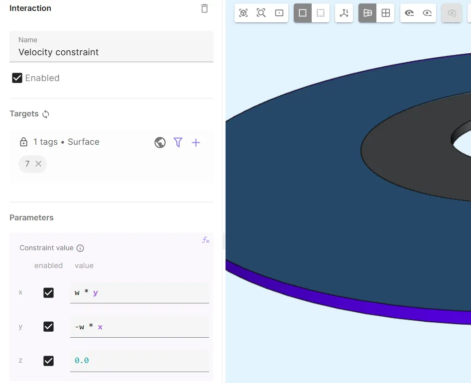
- As Target, select the water cylinder’s outer edge surface (
-
Add
Velocity constraint 2.- As Target, select the interface surface between the fluid and solid regions (
4). - Set Constraint value to
[1, 0; 1, 0; 1, 0]. - This is essentially a no-slip constraint at the fluid and solid interface.
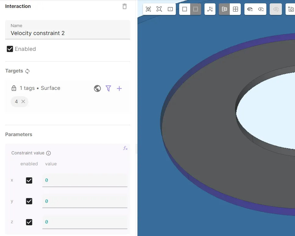
- As Target, select the interface surface between the fluid and solid regions (
-
Add
Velocity constraint 3.- As Target, select the water cylinder top and bottom surfaces (
8, 9). - Set Constraint value to
[0, 0; 0, 0; 1, 0].
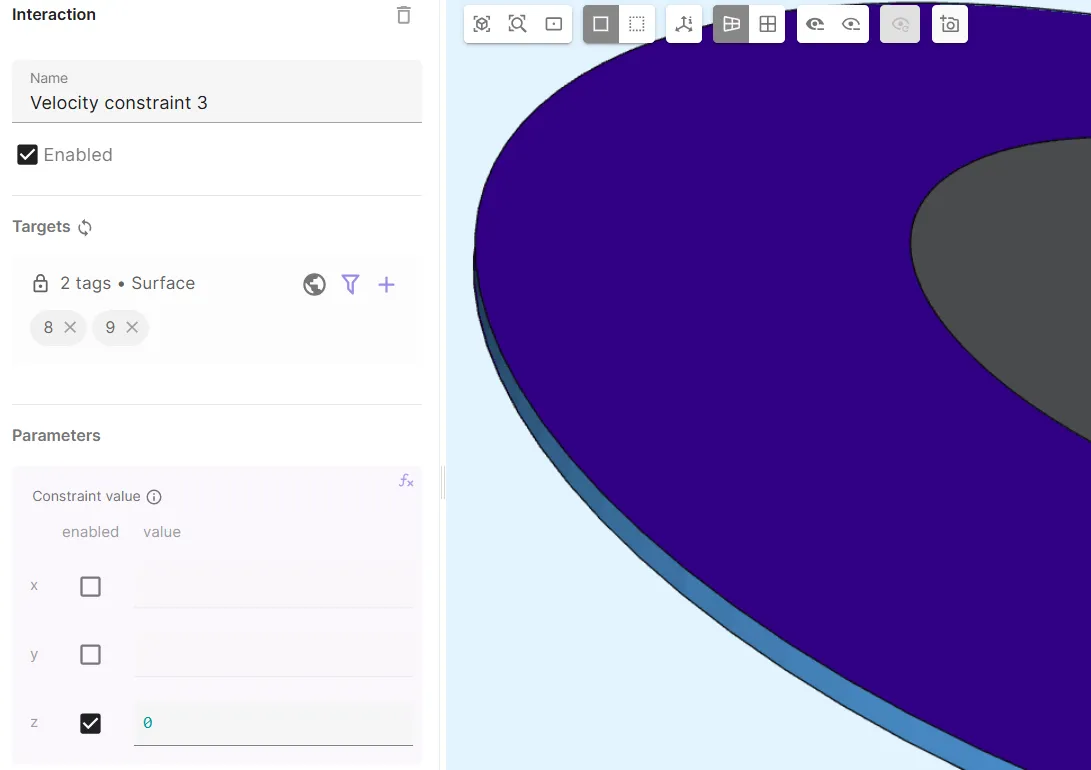
- This constraint stops flow in the Z-direction through the water cylinder top and bottom surfaces.
- This is what makes the simulation quasi-2D as the velocity in the Z-direction is set to zero.
- As Target, select the water cylinder top and bottom surfaces (
-
Add
Pressure constraint.- As Target, select points
3, 4. - Set Constraint value to
0.0.
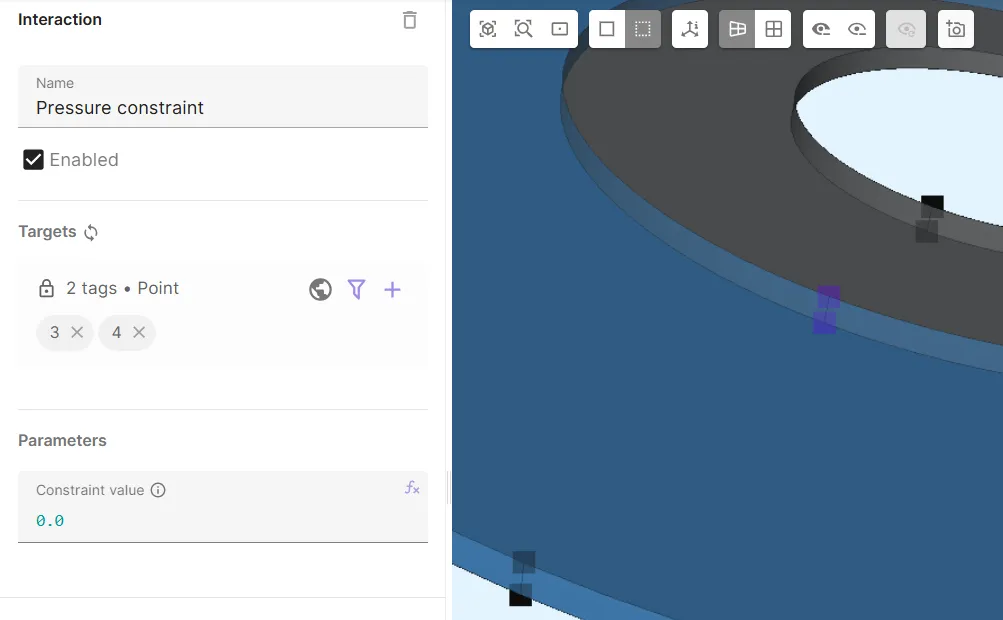
- As Target, select points
-
Add the Laminar flow - Heat fluid coupling
Thermal fluid.
Physics 2 - Heat solid
Section titled “Physics 2 - Heat solid”- As Heat solid target, select the aluminium region.
- Add
Constraint.- As Target, select the aluminium cylinder inner surface (
1). - Set Temperature constraint to
Ti.
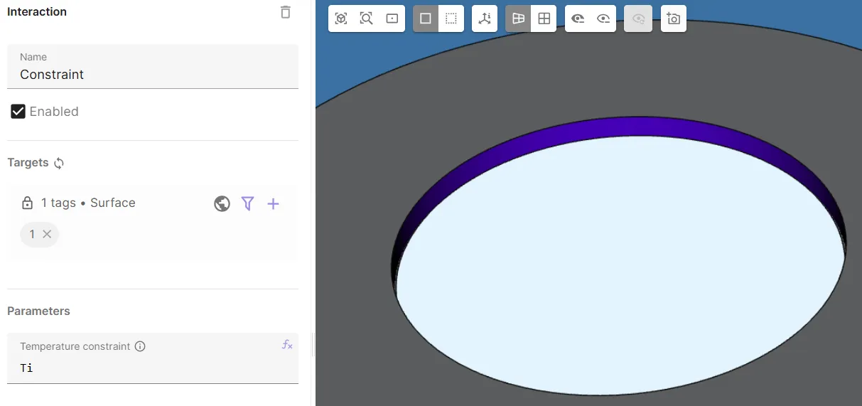
- As Target, select the aluminium cylinder inner surface (
Physics 3 - Heat fluid
Section titled “Physics 3 - Heat fluid”- As Heat fluid target, select the water region.
- Add
Constraint.- As Target, select the water cylinder outer surface (
7). - Set Temperature constraint to
To.
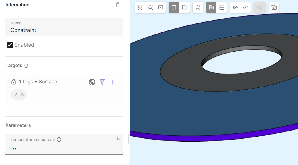
- As Target, select the water cylinder outer surface (
Your physics and their interactions are now defined.
Before moving on, check that your physics tree matches the one below.
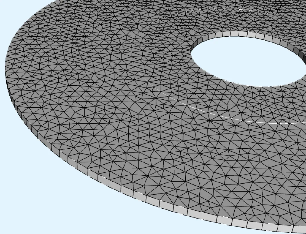
Step 5 - Generate the mesh
Section titled “Step 5 - Generate the mesh”Proceed to the Simulations section to create a new mesh.
For thin geometries like in here, it makes sense to use mesh extrusion:
- Set Mesh quality to
Expert settings. - Set Used mesher to
Basic. - Set Scale factor to
0.15. - Add Mesh extrusion.
- As Target, select both cylindrical volumes in the model (
2, 3). - This creates just one extrusion layer.
Set Sublayer count in that layer to
1. - Apply the settings and mesh.
- Check out the preview.
Finished mesh:
Step 6 - Simulate
Section titled “Step 6 - Simulate”In this step, we’ll look at:
- Setting up the static simulation
- How to calculate the analytical solution in your static simulation through scripting (optional)
- Setting up an additional sweep simulation (optional)
Static
Section titled “Static”Create a new simulation:
- In simulation settings:
- Set Analysis type to
Static. - Set Solver mode to
Iterative solver.
- Set Analysis type to
- In Mesh, select the mesh you created.
- In Outputs:
- Add pressure field output
p.- As Target, select the water region.
- Add velocity field output
V.- As Target, select the water region.
- Add temperature field output
T.
- Add pressure field output
Your static simulation is now ready to run.
Scripting the analytical solution
Section titled “Scripting the analytical solution”To calculate the analytical solution, add this snippet of code to the end of your static simulation.py script file:
################################################## VERIFICATION WITH ANALYTICAL SOLUTIONRo = expr.RoRm = expr.RmRi = expr.RiTo = expr.ToTi = expr.TiUo = expr.Uoksbykf = expr.ksbykf
# Analytical solution for velocitydef V(r): """https://www.researchgate.net/publication/303316864_Improving_a_conjugate-heat-transfer_immersed-boundary_method""" """https://www.princeton.edu/~gasdyn/Research/T-C_Research_Folder/Analytical_Solution.html""" if (r>Ro or r<Rm): return 0.0 else: vel = Uo * (Ro/r) * (r*r-Rm*Rm)/(Ro*Ro-Rm*Rm) return vel
# Analytical solution for temperaturedef T(r): """https://www.researchgate.net/publication/303316864_Improving_a_conjugate-heat-transfer_immersed-boundary_method""" if (r >= Ri and r <= Rm): temp = Ti + (To-Ti) * qs.log(r/Ri) / (qs.log(Rm/Ri)+qs.log(Ro/Rm)*ksbykf) return temp.evaluate() elif (r >= Rm and r <= Ro): temp = To - (To-Ti) * qs.log(Ro/r) / (qs.log(Ro/Rm)+qs.log(Rm/Ri)/ksbykf) return temp.evaluate() else: return 0.0
rT = RmTinterface_analytical = T(rT)Tinterface_simulation = (fld.T).allinterpolate(qs.selectall(), [0, rT, 0])[0]
rV = (Ro + Rm)/2.0V_analytical = V(rV)V_simulation = (fld.V).allinterpolate(qs.selectall(), [0, rV, 0])[0]
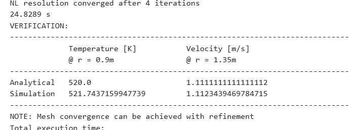
if(qs.getrank()==0): str_rT = f"@ r = {rT}m"; str_rV = f"@ r = {rV}m" print(f"{'VERIFICATION:'}", flush=True) print(f"{'':-^75}", flush=True) print(f"{'':12} {'Temperature [K]':<25} {'Velocity [m/s]':<25}", flush=True) print(f"{'':12} {str_rT:<25} {str_rV:<25}", flush=True) print(f"{'':-^75}", flush=True) print(f"{'Analytical':<12} {Tinterface_analytical:<25} {V_analytical:<25}", flush=True) print(f"{'Simulation':<12} {Tinterface_simulation:<25} {V_simulation:<25}", flush=True) print(f"{'':-^75}", flush=True)
print("NOTE: Mesh convergence can be achieved with refinement")#################################################See Logs for verification results:
Create a new simulation by copying the existing static simulation:
- Name the simulation copy as
Sweep. - In Inputs:
- Add
ksbykf sweep.- Set Override expression to
linspace(0.1, 20, 40).
- Set Override expression to
- Add
- In Outputs:
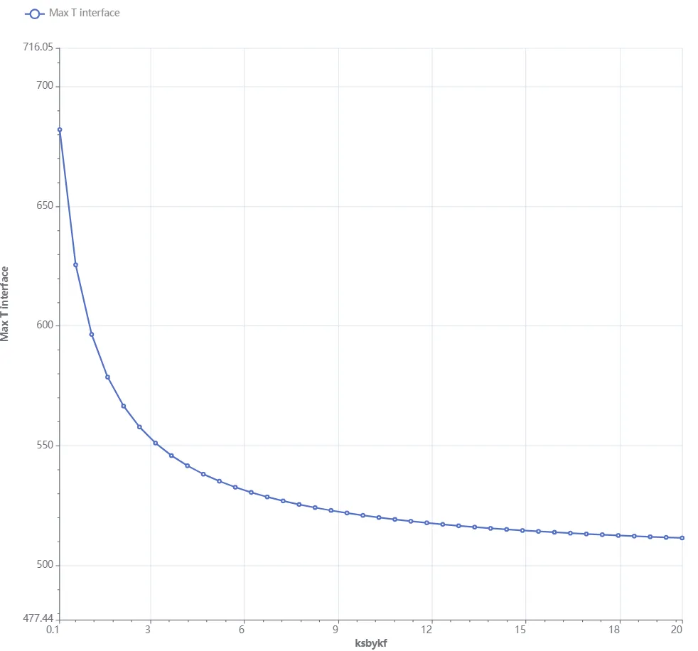
- Add custom value output:
- Name:
Max T interface. - Output expression:
maxvalue(reg.interface_surface, T, 5).
- Name:
- Add custom value output:
- Name:
FSI flux. - Output expression:
integrate(reg.interface_surface, transpose(normal(reg.aluminium)) * on(reg.aluminium, -par.k()*grad(T)), 5).
- Name:
- Add custom value output:
Your sweep simulation is now ready to run.
Step 7 - Plot & visualize
Section titled “Step 7 - Plot & visualize”In the Simulations section, add plots to see value output results, or visualizations to see field output results.
Some examples are given below.
-
Temperature field T:
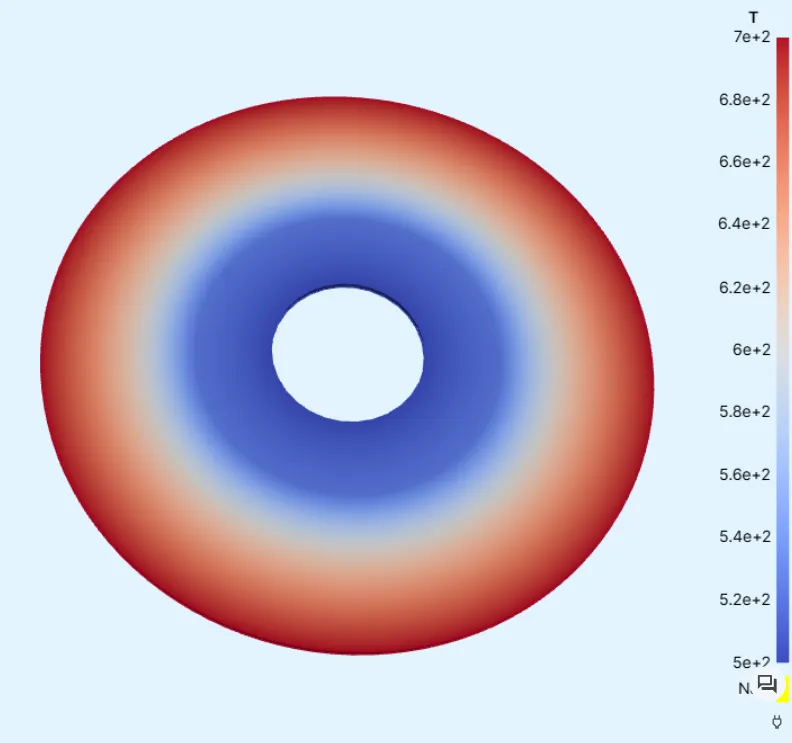
-
Max T interface:
Results
Section titled “Results”
References
Section titled “References”Footnotes
Section titled “Footnotes”-
De Marinis, D., de Tullio, M.D., Napolitano, M. and Pascazio, G. (2016). Improving a conjugate-heat-transfer immersed-boundary method. International Journal of Numerical Methods for Heat & Fluid Flow, Vol. 26 No. 3/4, pp. 1272-1288. https://doi.org/10.1108/HFF-11-2015-0473> ↩