Pull-in analysis of a MEMS device
In this tutorial, pull-in analysis is simulated for a MEMS device.
Pull-in analysis is performed to determine the pull-in voltage of a MEMS device. At this voltage, the device becomes unstable as the electrostatic forces can no longer be balanced by the stiffness of the device.
Model definition
Section titled “Model definition”The model consists of two parallel square plates with a certain thickness, separated by a vacuum gap. A DC voltage is applied to the bottom plate while the top plate is grounded. The bottom plate is clamped and the top plate is attached to a spring with stiffness . The displacement of the top plate is constrained to move only in the -direction. The interaction between the top plate and attached spring is determined using a lumped model:

Parameters
Section titled “Parameters”The model parameters, that should be defined as variables in Allsolve, are defined as follows:
- Length of the square plate, μm
- Height of the square plate, μm
- Gap between the two parallel square plates, μm
- Stiffness of the spring, N/m
- Overlapping area between the two parallel plates, m²
Geometric elements
Section titled “Geometric elements”| Element | Size | Center point (X, Y, Z) |
|---|---|---|
| Bottom plate | L L H | (0, 0, 0) |
| Top plate | L L H | (0, 0, H + d) |
| Vacuum box | L L d | (0, 0, H/2 + d/2) |
Output Results
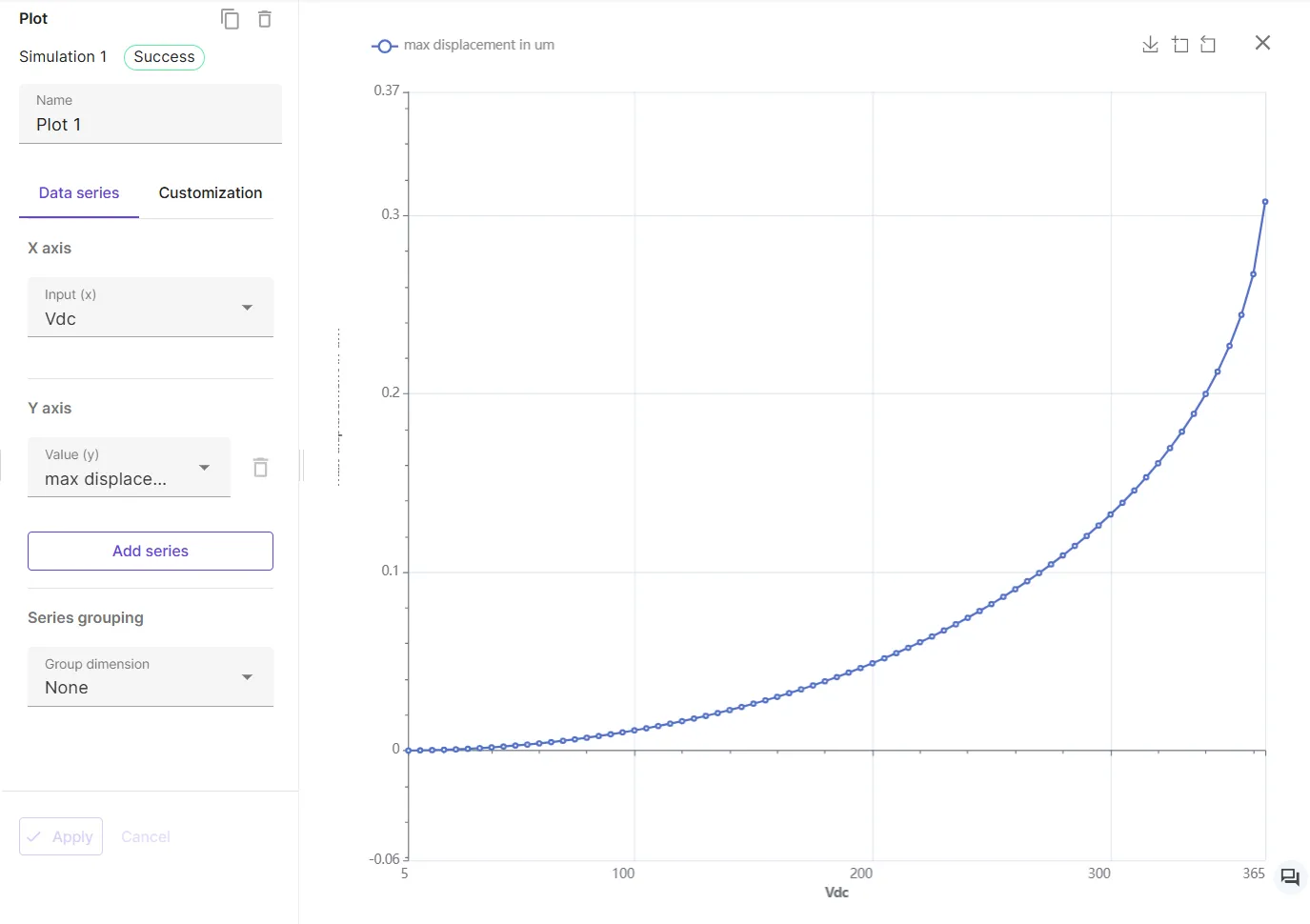
Section titled “Output Results”- Plot of applied voltage vs resulting displacement.
Material Data
Section titled “Material Data”- Vacuum for the gap between the parallel plates
- Electric permittivity: = [F/m]
- Silicon dioxide for the top and bottom plate
- Young’s modulus: = [GPa]
- Poisson’s ratio: =
- Electric permittivity: = [F/m]
Boundary conditions
Section titled “Boundary conditions”-
Bottom plate
- Electrode: =
- Clamped: =
-
Top plate
- Grounded: =
- in-plane clamp: =
Analytical solution
Section titled “Analytical solution”For the model setup defined above, the analytical solution to the pull-in voltage is given by the formula: 1
where,
- is the spring stiffness [N/m].
- is the initial gap between the parallel plates [m].
- is the electric permittivity of the gap medium [F/m].
- is the overlapping area between the parallel plates [m²].
The corresponding displacement of the top plate at pull-in voltage is one-third of the initial gap between the plates.
The pull-in voltage and the corresponding displacement based on the values defined in Parameters:
Step-by-step guide
Section titled “Step-by-step guide”Here you’ll find a detailed step-by-step tutorial on how to simulate this in Quanscient Allsolve
Step 1 - Build the geometry
Section titled “Step 1 - Build the geometry”-
Start with a new project, and name it as
Pull-in analysis. -
In the project starting options dialog, choose
boxas a starting point. -
Finish model editing for now and go to the
Commonsidebar. -
Add variables:
Name Description Expression L Plate size [m] 50e-6H Plate thickness [m] 3e-6d Gap between plates [m] 1e-6Vdc DC Voltage [V] 1K Spring stiffness [N/m] 1e4A Overlap area between plates [m] L*L -
Go back to the
Geometrysection to finish model editing. -
Change the box size (X; Y; Z) to (
L;L;H):Name Element type Center point [m] Size [m] Rotation [deg] box Box X: 0X: LX: 0Y: 0Y: LY: 0Z: 0Z: HZ: 0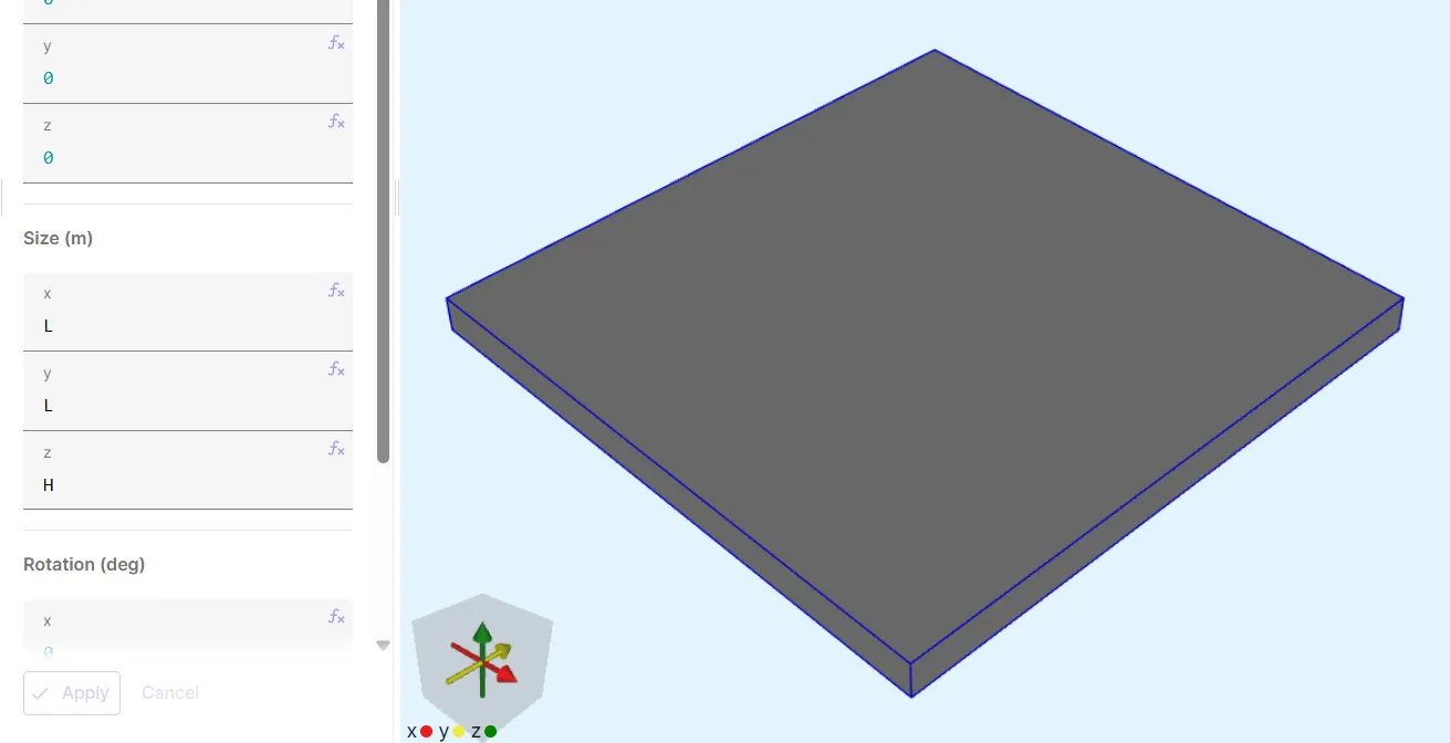
-
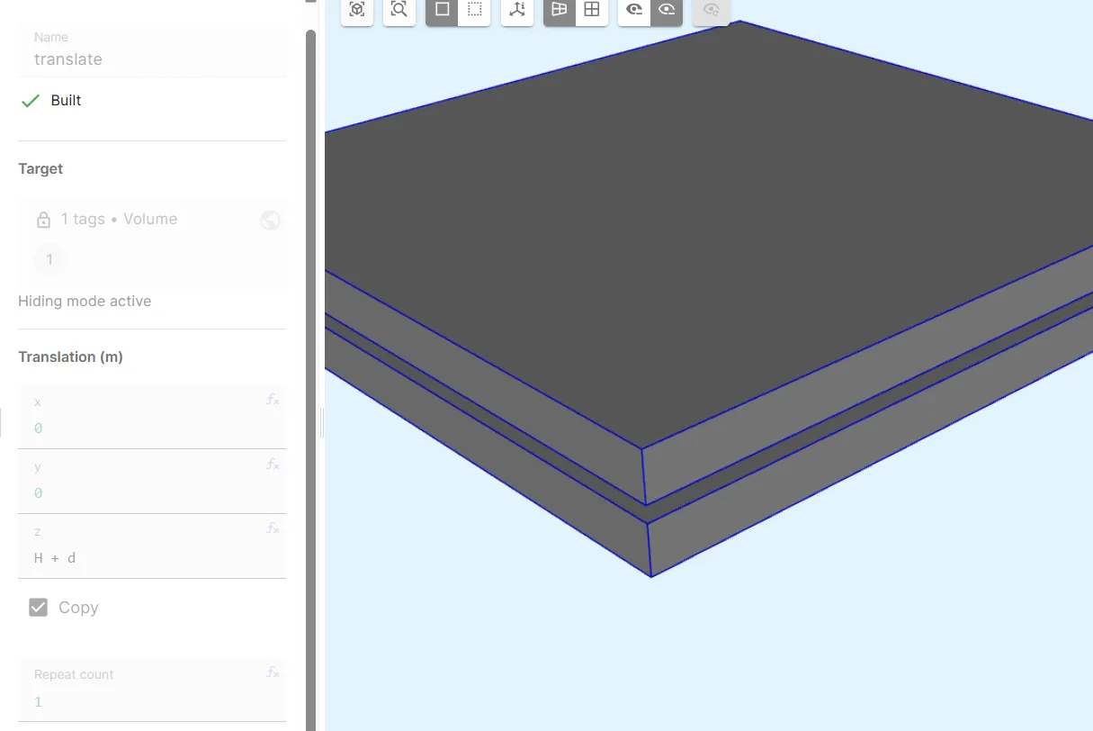
To build the other parallel plate, use the
Translategeo operation:Name Element type Target Translation [m] Copy Repeat count translate Translation Volume 1X: 0Yes 1Y: 0Z: H + d -
Confirm the settings and build the translation.
-
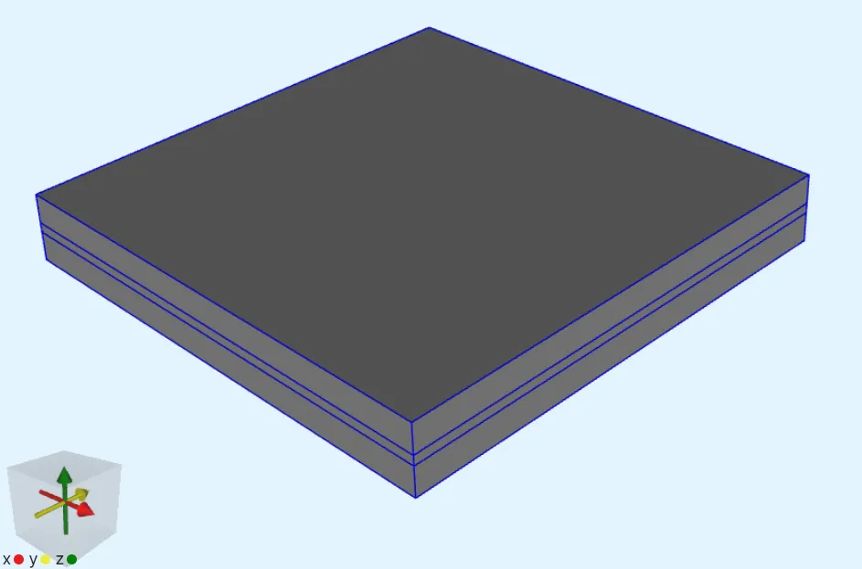
To fill the gap between the parallel plates, build another box:
Name Element type Center point [m] Size [m] Rotation [deg] box 2 Box X: 0X: LX: 0Y: 0Y: LY: 0Z: H/2 + d/2Z: dZ: 0
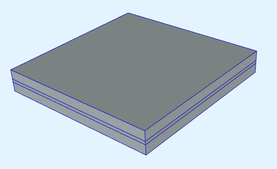
Your geometry is now finished.
Step 2 - Define the materials
Section titled “Step 2 - Define the materials”-
Go to the
Commonsidebar. -
Add the
Vacuummaterial and assign it to the gap between the plates (volume25). Add the target region as a shared region. -
Add the
Silicon dioxidematerial and assign it to the plates (volumes1, 2). Add the target as a shared region.
Step 3 - Define physics and interactions
Section titled “Step 3 - Define physics and interactions”-
Go to the
Physicssection. -
Add the
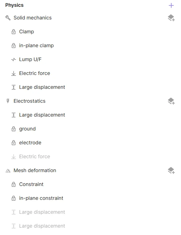
Solid Mechanics,ElectrostaticsandMesh deformationphysics.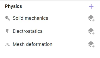
Physics 1 - Solid mechanics
Section titled “Physics 1 - Solid mechanics”-
Select the silicon dioxide shared region (volumes
1, 2) as solid mechanics target.Physics Target Solid mechanics Silicon dioxide region (volumes 1, 2) -
Add a
Clampinteraction to Solid mechanics.Interaction name Interaction type Target Value Clamp ClampBottom plate (volume 1) -
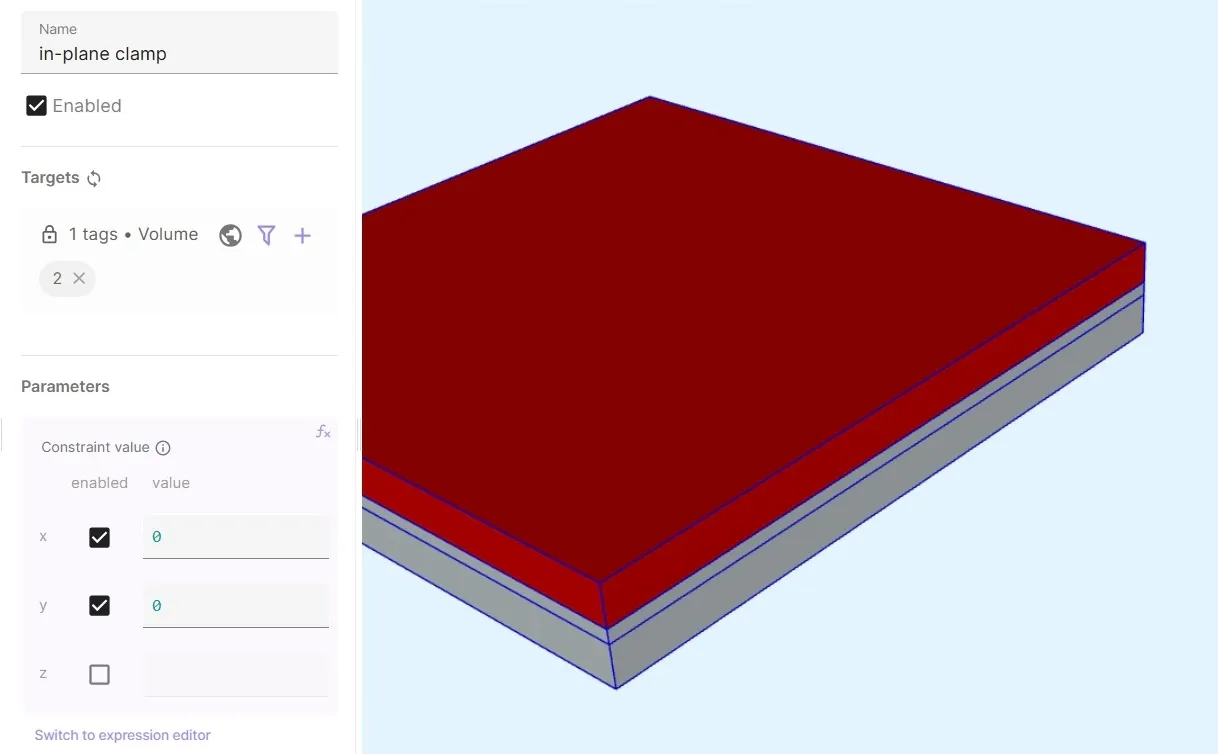
Add a
Constraintinteraction to Solid mechanics:Interaction name Interaction type Target Value in-plane clamp ConstraintTop plate (volume 2)[1, 0; 1, 0; 0, 0]The in-plane clamp interaction is used to constraint the movement of the top plate in X and Y directions. Z-directional movement is left unconstrained.
-
Add
Lump U/Fto Solid mechanics:Interaction name Interaction type Target Actuation mode Value Lump U/F Lump U/FTop plate top surface (surface 12)Circuit coupling[0, 0; 0, 0; 1, lump.Fz + K*lump.Uz]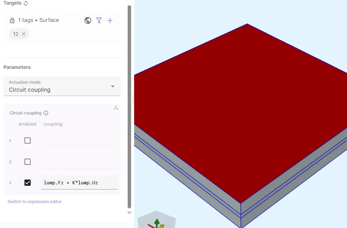
Lump U/F is used to attach a spring to the top surface of the top plate via circuit coupling.
-
Add the
Electric forceinteraction, which couples Solid mechanics to Electrostatics. -
Add the
Large displacementinteraction, which couples Solid mechanics to Mesh deformation.
Physics 2 - Electrostatics
Section titled “Physics 2 - Electrostatics”-
Let the electrostatics target default to the whole geometry.
Physics Target Electrostatics All volumes ( 1, 2, 25) -
Add a
Constraintinteraction to Electrostatics.Interaction name Interaction type Target Value ground ConstraintTop plate (volume 2)0 -
Add another
Constraintinteraction to Electrostatics:Interaction name Interaction type Target Value electrode ConstraintBottom plate (volume 1)Vdc -
Add the
Large displacementinteraction, which couples Electrostatics to Mesh deformation.
Physics 3 - Mesh deformation
Section titled “Physics 3 - Mesh deformation”-
Let the mesh deformation target default to the whole geometry.
Physics Target Mesh deformation All volumes ( 1, 2, 25) -
Add a
Constraintinteraction to Mesh deformation:Interaction name Interaction type Target Value Constraint ConstraintSilicon dioxide target (volumes 1, 2)[1, compx(u); 1, compy(u); 0, compz(u)]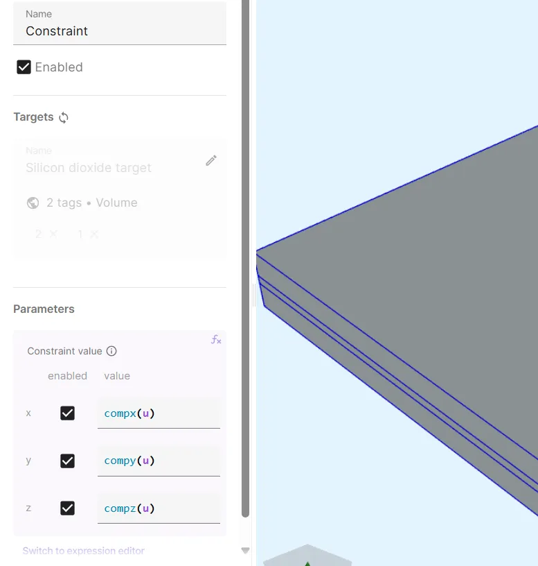
-
Add another
Constraintinteraction to Mesh deformation:Interaction name Interaction type Target Value in-plane constraint ConstraintVacuum gap (volume 25)[1, 0; 1, 0; 0, 0]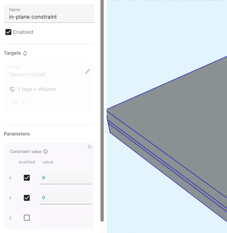
All your physics and interactions are now added.
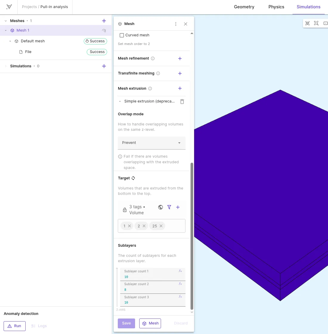
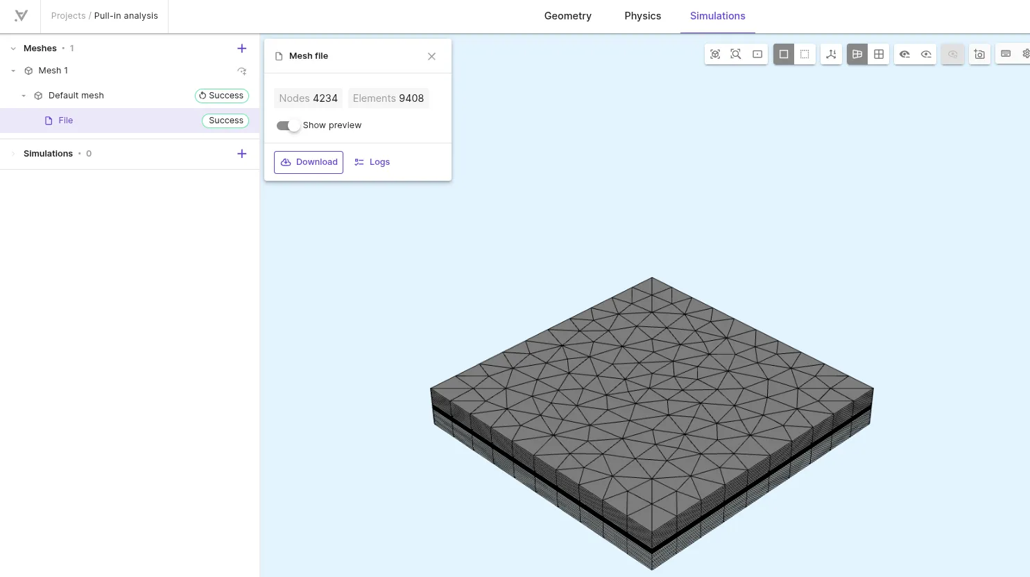
Step 4 - Generate the mesh
Section titled “Step 4 - Generate the mesh”-
Go to the
Simulationssection. -
Add a new mesh.
-
Set Mesh quality to
Expert Settings. -
Set Used Mesher to
Basic. -
Set Scale factor to
0.75. -
Add
Mesh extrusion:Mesh entity Overlap mode Target Sublayer counts Mesh extrusion PreventAll volumes 1, 2, 2510810 -
Run meshing and check the preview.
Step 5 - Apply settings and run the simulation
Section titled “Step 5 - Apply settings and run the simulation”-
Add a new simulation.
-
Set Analysis Type to
Static. -
Select the mesh you created in Step 4 as the mesh for your simulation.
-
Add a
Vdc sweepinput with override expressionlinspace(5, 365, 73). -
Add a custom value output and name it as
max displacement in um. Set Output expression tomaxvalue(reg.silicon_dioxide_target, -compz(u), 5) * 1e6. -
The Solid mechanics physics considers geometric nonlinearity due to the Large displacement interaction. It is sufficient to consider geometric linearity for this simulation. To make this change, open the script and toggle on
Scripting mode. -
Scroll down to
# Solid mechanicsin the script, and replace the formulation with the line below:form += qs.integral(reg.silicon_dioxide_target, qs.predefinedelasticity(qs.dof(fld.u), qs.tf(fld.u), par.H()))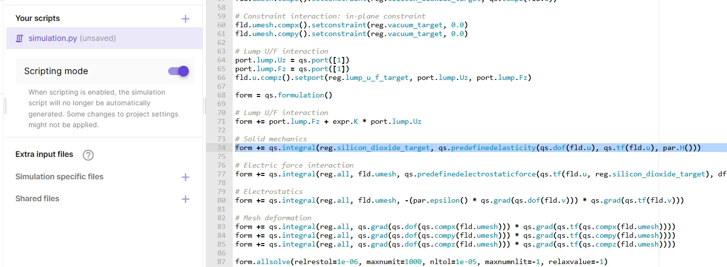
Your settings are now applied, and you can run the simulation.
Step 5 - Plot results
Section titled “Step 5 - Plot results”Add a plot with Vdc in the X axis, and max displacement in um in the Y axis.
References
Section titled “References”Footnotes
Section titled “Footnotes”-
Kaajakari, V. MEMS Tutorial: Pull-in voltage in electrostatic microactuators, 1-2. https://www.kaajakari.net/~ville/research/tutorials/pull_in_tutorial.pdf ↩