EM 002 – IM 2D torque analysis
In this demo, we perform a transient simulation from a 2D cross-section of an Induction Motor (IM), using the H–φ formulation [2]. We also validate results against the Compumag TEAM (Testing Electromagnetic Analysis Methods) Problem 30 [1].
Induction motors are widely used in industrial applications due to their robustness, low cost, and simple construction.
Model Definitions
Section titled “Model Definitions”Induction Motor
Section titled “Induction Motor”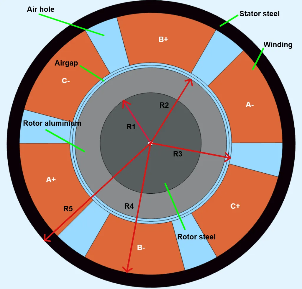
| Radius | Value (cm) |
|---|---|
| R1 | 2.0 |
| R2 | 3.0 |
| R3 | 3.2 |
| R4 | 5.2 |
| R5 | 5.7 |
The motor has six stator windings, each phase covering 45°. The air region between each copper winding phase is 15°.
The + and – signs describe the direction of the three-phase currents.
We will go step-by-step through the solution process in Quanscient Allsolve.
Step 1 – Build the Geometry
Section titled “Step 1 – Build the Geometry”-
Create a 2D project and import the
.STEPfile of the induction motor cross-section:
induction-motor-2D-team30.step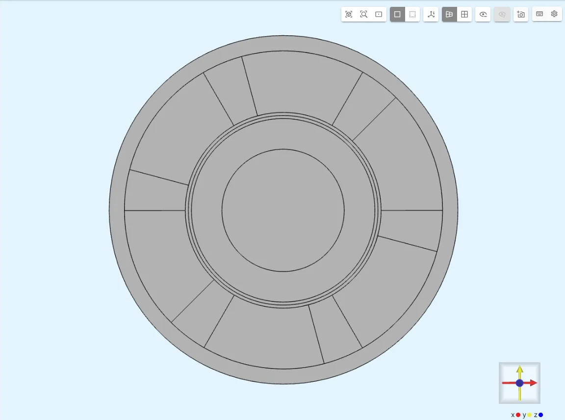
-
Create two disks:
Hole: the rotor’s central shaft hole.Surroundings: the surrounding air region.
Disk Name Center X (m) Center Y (m) Size (m) Hole0.0 0.0 0.001 Surroundings0.0 0.0 0.30 -
Use Fragment All to clean up the geometry.
-
Remove the
Holeusing the Difference operation:Parameter Surfaces Set 1 All surfaces Set 2 Hole(Delete = ✔ Enabled) -
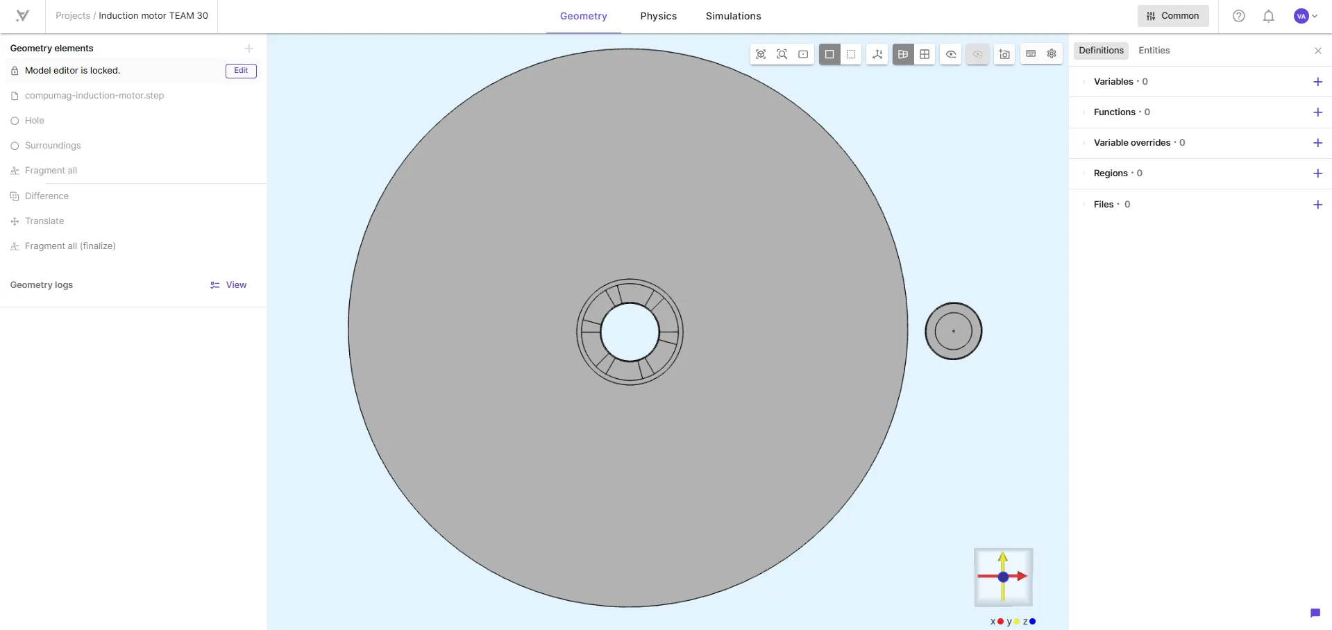
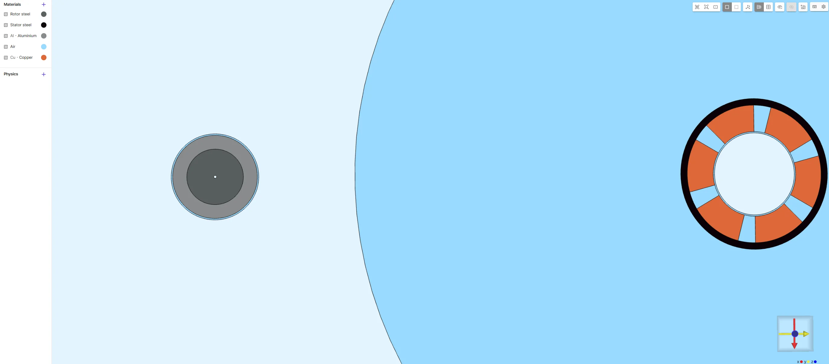
Translate the rotor outward (e.g.,
0.35 malong the x-axis) for separate meshing. Disable the Copy option.
After confirming the model changes, your geometry should look like this:
Step 2 – Apply Physics
Section titled “Step 2 – Apply Physics”Define Surface Regions
Section titled “Define Surface Regions”Navigate to: Common → Definitions → Region → Surface
Define the following surface regions:
| Region Name | Notes | Tags |
|---|---|---|
rotor | Rotor steel, rotor aluminium, and rotor side airgap slice | 72-74 |
airgap | Rotor and stator side airgap slices | 17, 74 |
magnetism_H | All windings and rotor aluminium | 10-15, 73 |
magnetism_phi | Rotor/stator steel, airgap, air holes, and surrounding air | 4-9, 16-17, 71-72, 74 |
Assign Materials
Section titled “Assign Materials”| Part | Material | Name | Electric conductivity [S/m] | Magnetic permeability [H/m] |
|---|---|---|---|---|
| Rotor steel | Carbon Steel AISI 1020 | Rotor steel | 1.6e6 | 30*mu0 |
| Stator steel | Carbon Steel AISI 1020 | Stator steel | 0 | 30*mu0 |
| Windings | Copper | Copper | 1 | mu0 |
| Rotor aluminium | Aluminium | Aluminium | 3.72e7 | mu0 |
| Airgap, air holes, surroundings | Air | Air | 0 | mu0 |
Define Simulation Variables
Section titled “Define Simulation Variables”Navigate to:
Common → Definitions → Variables and add New variables:
| Name | Description | Value |
|---|---|---|
I_max | Max current [A] | 2045.175 |
rpm | Rotor speed [rpm] | 0 |
Step 3 – Add Magnetism φ Interactions
Section titled “Step 3 – Add Magnetism φ Interactions”- Apply
Magnetism φto all parts except copper windings and rotor aluminium.
Gauge Constraint
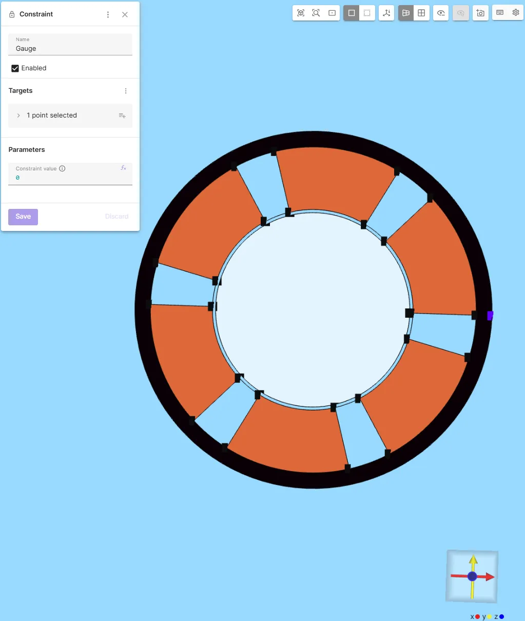
Section titled “Gauge Constraint”- Add a
Constraintto ensure a unique solution.
Setvalue = 0at a point on the outer edge of stator.
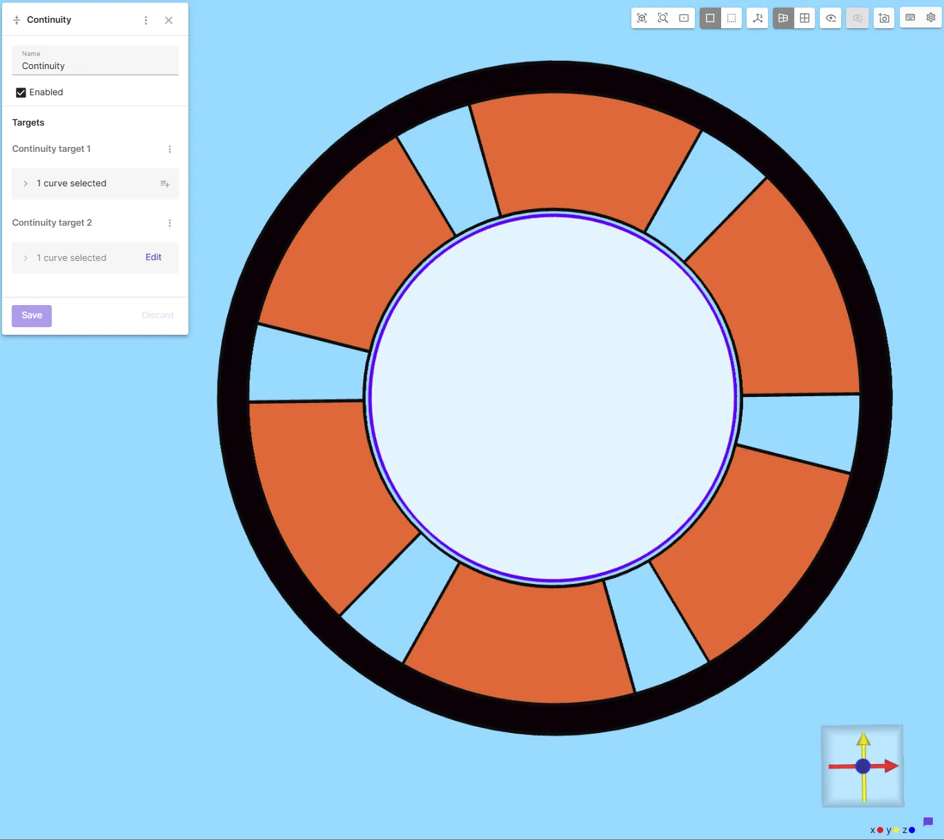
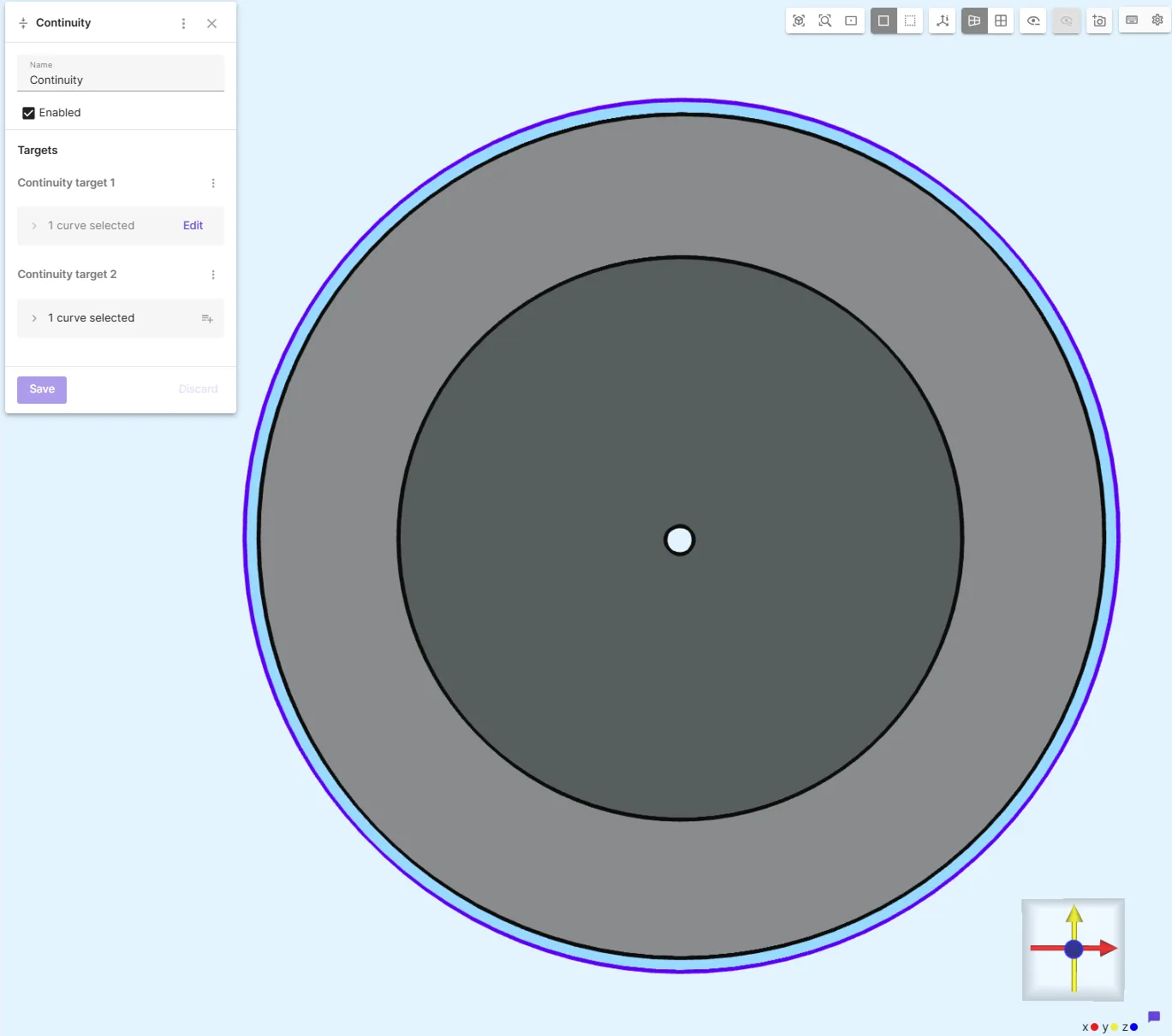
Airgap Continuity
Section titled “Airgap Continuity”- Add
Continuityacross the rotor–stator interface:- Target 1 = stator side curve
- Target 2 = rotor side curve
(Order matters!)
Stator side:
Rotor side:
Apply Stator Currents
Section titled “Apply Stator Currents”To create a rotating magnetic field, we apply phase currents to the windings using Lump I/V cut interactions.
1. Define the Phase Interactions
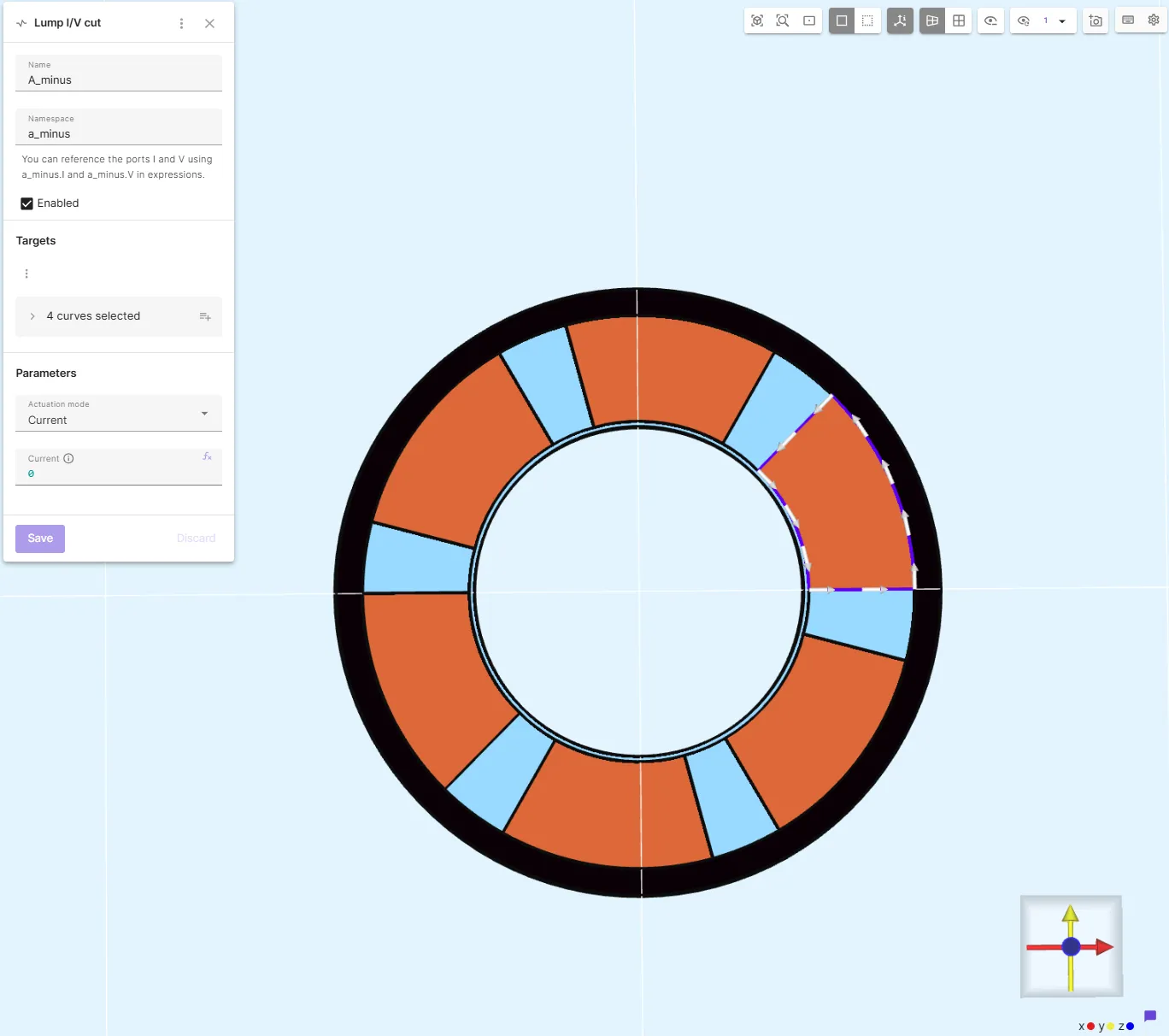
Section titled “1. Define the Phase Interactions”Add Lump I/V cut interactions by selecting the 4 boundary curves for each winding, and using the namespaces below:
| Phase | Namespace | Current |
|---|---|---|
| A− | a_minus | 0 |
| B+ | b_plus | 0 |
| C− | c_minus | 0 |
| A+ | a_plus | 0 |
| B− | b_minus | 0 |
| C+ | c_plus | 0 |
For now, set all Current values to 0 — we’ll define them later via scripting.
2. Verify Lump Curve Orientation
Section titled “2. Verify Lump Curve Orientation”Ensure each lump curve is oriented counter-clockwise within its phase winding, as shown below:
3. Add Net Current Constraint
Section titled “3. Add Net Current Constraint”Finally, add a Lump I/V cut interaction to the small central hole.
This enforces a net zero current constraint on induced currents in the rotor aluminium.
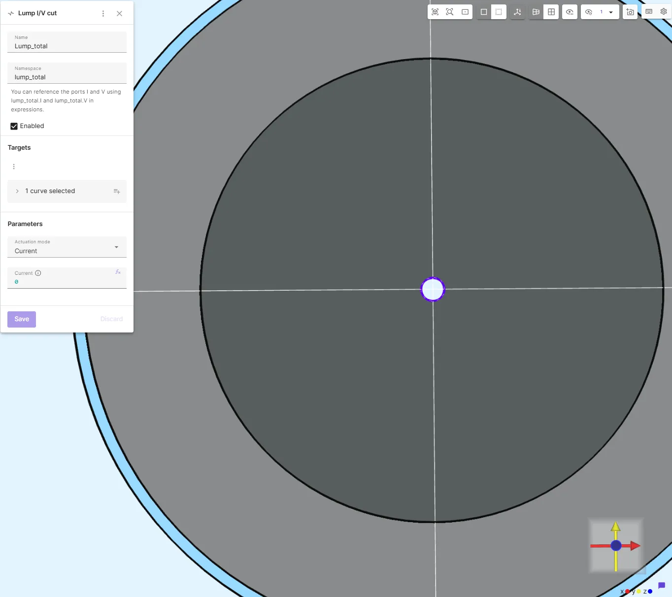
Set:
- Namespace =
lump_total Current = 0
Step 4 – Add Magnetism H Interactions
Section titled “Step 4 – Add Magnetism H Interactions”- Apply
Magnetism Hto copper windings and rotor aluminium. - Couple
Magnetism HwithMagnetism φ.
Step 5 – Mesh Settings
Section titled “Step 5 – Mesh Settings”Go to Simulations → Meshes, and
- Switch
Mesh qualityto Expert settings. - Enable Curved mesh and Mesh refiner.
Mesh refinements:
| Surface | Max size (m) |
|---|---|
airgap | 0.0003 |
Surroundings | 0.02 |
Stator steel | 0.003 |
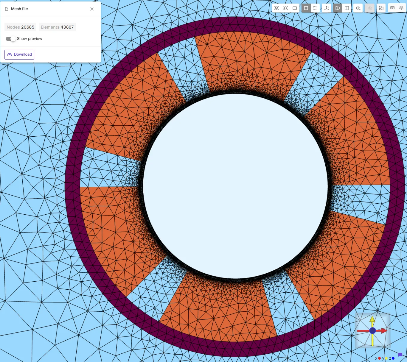
Example meshes:
Rotor mesh:
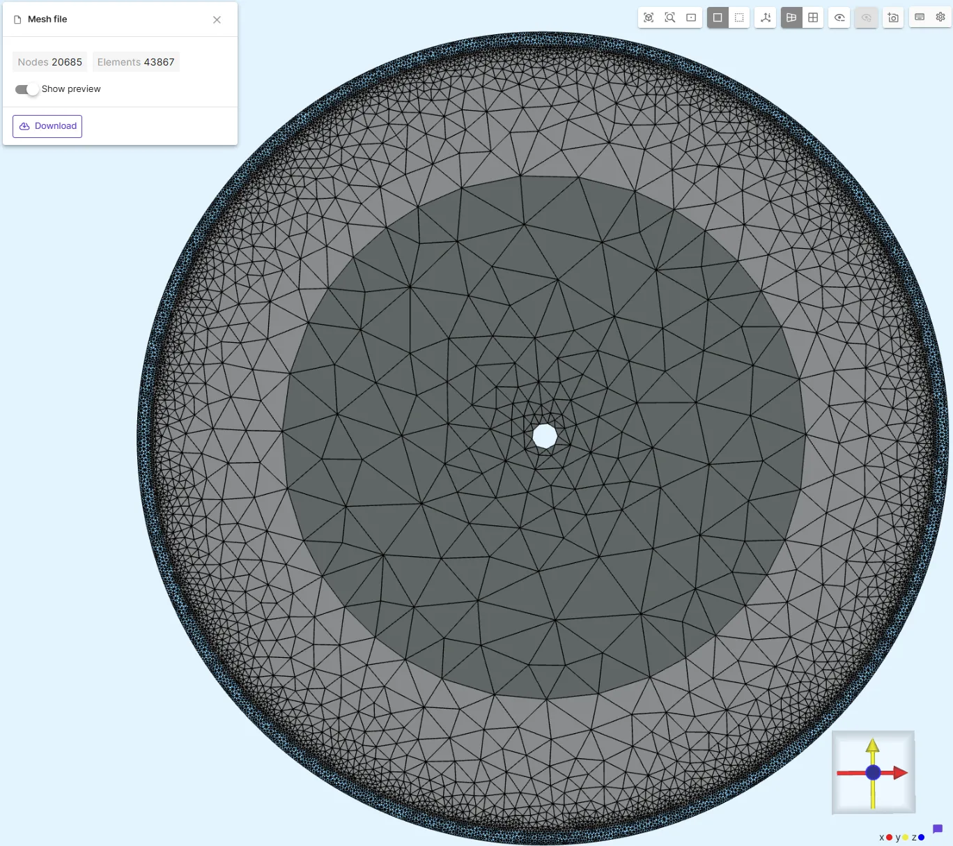
Stator mesh:
Step 6 – Simulation Setup
Section titled “Step 6 – Simulation Setup”- Set Analysis Type to
Transient
- Timestep algorithm: Implicit Euler
- Start time:
0 - End time:
1 - Timestep:
0.1
- Enable
Magnetism φandMagnetism H. - Add the generated mesh.
- Keep other settings as default.
Step 7 – Script Modifications
Section titled “Step 7 – Script Modifications”Next, we got to the Script section and enable Full scripting mode.
The following modifications allow dynamic rotor motion, correct 3D vector handling in a 2D model, and proper winding current definitions.
To simulate rotor movement dynamically, first reverse the initial static translation.
Insert the following lines right after the mesh.mesh.load() call:
# Reverse rotor shifttranslation_x = 0.35mesh.mesh.shift(reg.rotor, -translation_x, 0.0, 0.0)Adapt Field Vectors for 3D Calculations
Section titled “Adapt Field Vectors for 3D Calculations”Although this is a 2D simulation, the solver’s algorithms use 3D vectors. Therefore, we must update some of the default 2x1 vectors to 3x1 vectors by adding a zero to the z-dimension.
First, modify the parameter definitions for the magnetic field components:
df.H = qs.parameter(3, 1) # Magnetic field vector (Hx, Hy, Hz=0)df.B = qs.parameter(3, 1) # Magnetic flux density vectordf.j = qs.parameter(3, 1) # Current density vectordf.E = qs.parameter(3, 1) # Electric field vectorDecrease field order
Section titled “Decrease field order”Decrease field order from 2 → 1 for faster simulation:
# Magnetic scalar potential fieldfld.phi = qs.field("h1")fld.phi.setorder(reg.all, 1)Next, update the Magnetic field and Magnetic flux density definitions. This involves resizing the gradient of the magnetic scalar potential (fld.phi) and converting the remanence flux density arrays from qs.array2x1 to qs.array3x1.
Magnetic field
Section titled “Magnetic field”df.H.addvalue(qs.selectunion([reg.magnetism_h, reg.magnetism_phi]), -qs.grad(fld.phi).resize(3,1))df.H.addvalue(reg.magnetism_h, fld.H)df.H.addvalue(qs.selectunion([reg.magnetism_h, reg.magnetism_phi]), var.Hs)Magnetic flux density
Section titled “Magnetic flux density”df.B.addvalue(qs.selectunion([reg.magnetism_h, reg.magnetism_phi]), -par.mu() * qs.grad(fld.phi).resize(3,1))df.B.addvalue(reg.magnetism_h, par.mu() * fld.H)df.B.addvalue(qs.selectunion([reg.magnetism_h, reg.magnetism_phi]), par.mu() * var.Hs)Define Winding Currents
Section titled “Define Winding Currents”To generate a rotating magnetic field, you must define the sinusoidal currents for each phase of the motor windings. The following code block sets up three-phase currents (A, B, C) with a 120 degree phase shift.
Replace the entire auto-generated Lump I/V cut interactions section with the code below. This assumes the windings were created and named with identical namespaces.
f = 60 # [Hz]omega = 2*math.pi*f # [rad/s]I_rms = math.sqrt(2)*expr.I_max # [A]
# 3-phase currents 120 degrees offsetA = 0B = 2*math.pi/3C = -2*math.pi/3
# Lump I/V cut interaction: A_minusform += port.a_minus.I - I_rms*qs.cos(omega*qs.t() + A)# Lump I/V cut interaction: B_plusform += port.b_plus.I + I_rms*qs.cos(omega*qs.t() + B)# Lump I/V cut interaction: C_minusform += port.c_minus.I - I_rms*qs.cos(omega*qs.t() + C)# Lump I/V cut interaction: A_plusform += port.a_plus.I + I_rms*qs.cos(omega*qs.t() + A)# Lump I/V cut interaction: B_minusform += port.b_minus.I - I_rms*qs.cos(omega*qs.t() + B)# Lump I/V cut interaction: C_plusform += port.c_plus.I + I_rms*qs.cos(omega*qs.t() + C)# Net current zero constraintform += port.lump_total.I - 0.0
Finally, resize the remaining gradient terms in the Magnetism φ and H-φ coupling interaction sections to ensure full 3D vector compatibility.
Magnetism φ
Section titled “Magnetism φ”# Magnetism φform += qs.integral(reg.magnetism_phi, -par.mu() * (qs.grad(qs.dof(fld.phi)).resize(3,1) - var.dof_Hs) * qs.grad(qs.tf(fld.phi)).resize(3,1))H-φ coupling
Section titled “H-φ coupling”# H-φ coupling interactionvar.phi_dofs_reg = qs.selectunion([reg.magnetism_phi, reg.magnetism_h])form += qs.integral(reg.magnetism_h, -par.mu() * qs.grad(qs.dt(qs.dof(fld.phi, var.phi_dofs_reg))).resize(3,1) * qs.tf(fld.H))form += qs.integral(reg.magnetism_h, -par.mu() * (qs.dt(qs.dof(fld.H)) + var.dt_dof_Hs - qs.grad(qs.dt(qs.dof(fld.phi, var.phi_dofs_reg))).resize(3,1)) * var.tf_Hs)form += qs.integral(reg.magnetism_phi, -par.mu() * (var.dt_dof_Hs - qs.dt(qs.grad(qs.dof(fld.phi))).resize(3,1)) * var.tf_Hs)form += qs.integral(reg.magnetism_h, par.mu() * (qs.dof(fld.H) - qs.grad(qs.dof(fld.phi, var.phi_dofs_reg)).resize(3,1) + var.dof_Hs) * qs.grad(qs.tf(fld.phi, var.phi_dofs_reg)).resize(3,1))Transient Parameters and Post-Processing
Section titled “Transient Parameters and Post-Processing”Replace all content after the H–φ coupling code block with the following script. This script configures:
- Appropriately sized time steps for the transient simulation
- Correct mesh rotation for each rotor speed (rpm)
- Torque computation using Arkkio’s method [3]
- Output of values, fields, and the reference solution
V_deg_per_s = 6 * expr.rpm   # Angular velocity in deg/s   ||  rpm = 360deg / 60s = 6 deg/sa = 7/11459b = 1 - adeg_step = a * expr.rpm + b
if (expr.rpm == 0):    V_deg_per_s = 6*1909    deg_step = 1
t_for_1_deg_step = deg_step/V_deg_per_s  # sec/(deg_step)
var.time_step = t_for_1_deg_stepvar.num_time_steps = 500var.start_time = 0.0var.end_time = var.num_time_steps*var.time_stepvar.step_index = 0.0
# Compute angle step in degrees per time stepangle_step = V_deg_per_s * var.time_step
timestepper = qs.impliciteuler(form, qs.vec(form))timestepper.settolerance(1e-05)timestepper.setrelaxationfactor(-1)qs.settime(var.start_time)
while qs.gettime() < var.end_time:    # Rotate mesh for amount the rpm rotation.    if (expr.rpm != 0):        mesh.mesh.rotate(reg.rotor, 0.0, 0.0, angle_step)
    timestepper.allnext(relrestol=1e-06, maxnumit=1000, timestep=var.time_step, maxnumnlit=1000)
    # 3-phase currents    qs.setoutputvalue("I_phase1", qs.evaluate(port.a_minus.I), qs.gettime())    qs.setoutputvalue("I_phase2", qs.evaluate(port.b_minus.I), qs.gettime())    qs.setoutputvalue("I_phase3", qs.evaluate(port.c_minus.I), qs.gettime())
    # J and B field outputs    qs.setoutputfield("J", reg.magnetism_h, df.j, 1, qs.gettime())    qs.setoutputfield("B", reg.all, df.B, 1, qs.gettime())
    # Net current should be approximately zero in rotor aluminium    qs.setoutputvalue("I_total ≈ 0 A", qs.allintegrate(reg.aluminium_target, qs.compz(df.j), 2), qs.gettime())
    dr = 0.002 # [m] airgap thickness    radius = qs.sqrt( qs.pow(qs.getx(),2) + qs.pow(qs.gety(),2) )    ephi = qs.array3x1(-qs.gety()/radius, qs.getx()/radius, 0)    er = qs.array3x1(qs.getx()/radius, qs.gety()/radius, 0)    Bphi = df.B*ephi    Br = df.B*er
    magforcedensity1 = (radius*Br*Bphi/qs.getmu0()/dr)    torque = magforcedensity1.allintegrate(reg.airgap, 2)    qs.setoutputvalue("Torque Arkkio [N*m]", qs.evaluate(torque), qs.gettime())
    var.step_index += 1
qs.setoutputvalue("Allsolve Torque [N*m]", qs.evaluate(torque))
rpms = [0, 1910, 3820, 5730, 7639, 9549, 11459]# Compumag valuesreference_vals = [3.825857, 6.505013, -3.89264, -5.75939, -3.59076, -2.70051, -2.24996]
# Function to set the torque based on RPMdef set_torque_for_rpm(rpm):    if rpm in rpms:        index = rpms.index(rpm)        qs.setoutputvalue("Reference torque [N*m]", reference_vals[index])    else:        raise ValueError(f"Unknown RPM value: {rpm}")
set_torque_for_rpm(expr.rpm)
Step 8 – Run a Simulation Sweep
Section titled “Step 8 – Run a Simulation Sweep”- Go to
Common → Definitions → Variable Overrides → Sweep. - Add a sweep for
rpmusing values:
[0, 1910, 3820, 5730, 7639, 9549, 11459](from Compumag TEAM Problem 30).
Step 9 – Run and Plot Results
Section titled “Step 9 – Run and Plot Results”- Include the sweep as an input to the simulation.
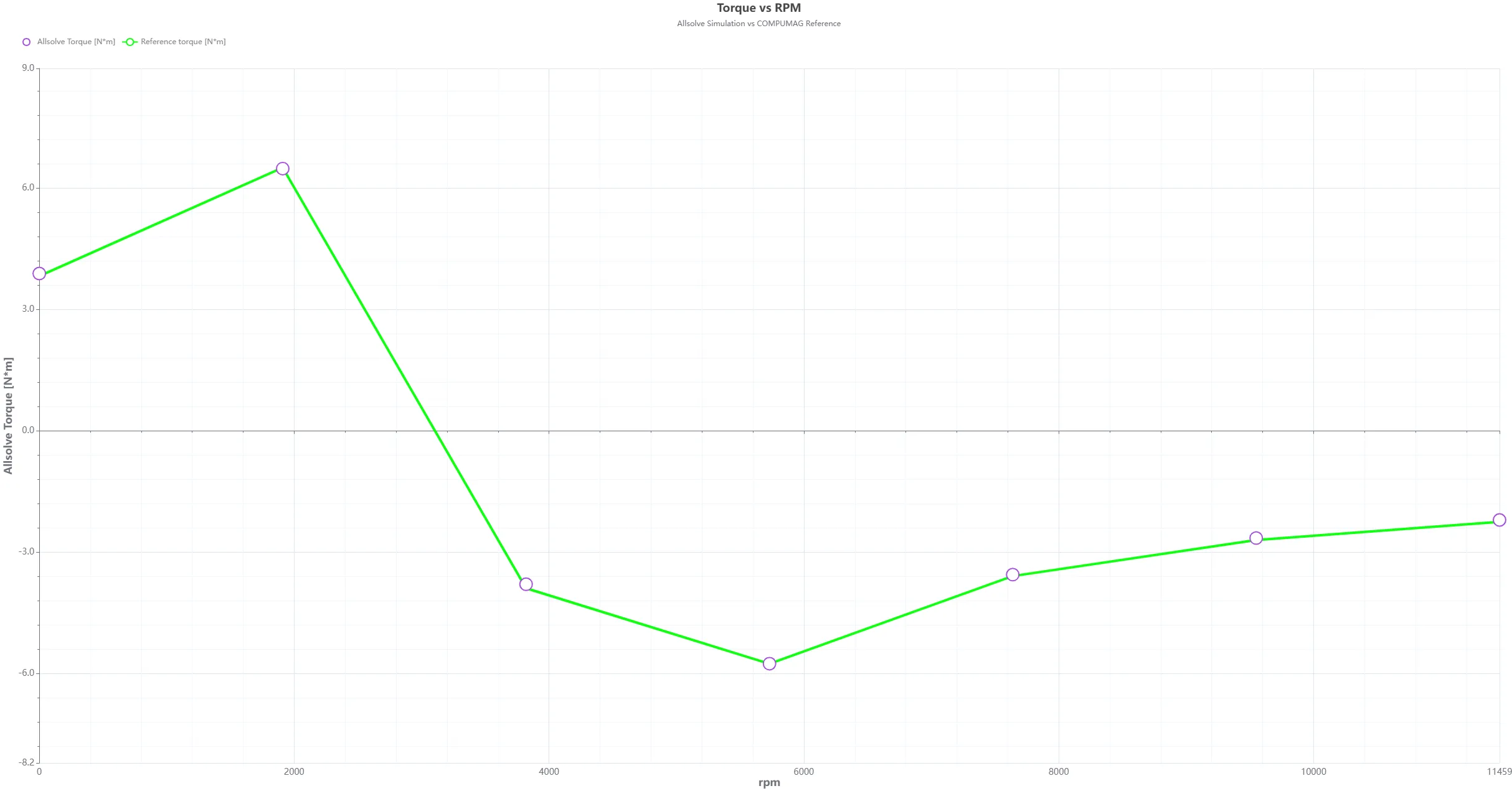
- Run the simulation and plot Torque vs. RPM.
The results should closely match the Compumag TEAM reference:
| Angular Speed (rad/s) | Speed (rpm) | Torque – Allsolve (N·m/m) | Torque – Reference (N·m/m) |
|---|---|---|---|
| 0 | 0 | 3.8897 | 3.8259 |
| 200 | 1910 | 6.4819 | 6.5050 |
| 400 | 3820 | -3.7942 | -3.8926 |
| 600 | 5730 | -5.7526 | -5.7594 |
| 800 | 7639 | -3.5552 | -3.5908 |
| 1000 | 9549 | -2.6508 | -2.7005 |
| 1200 | 11459 | -2.2035 | -2.2500 |
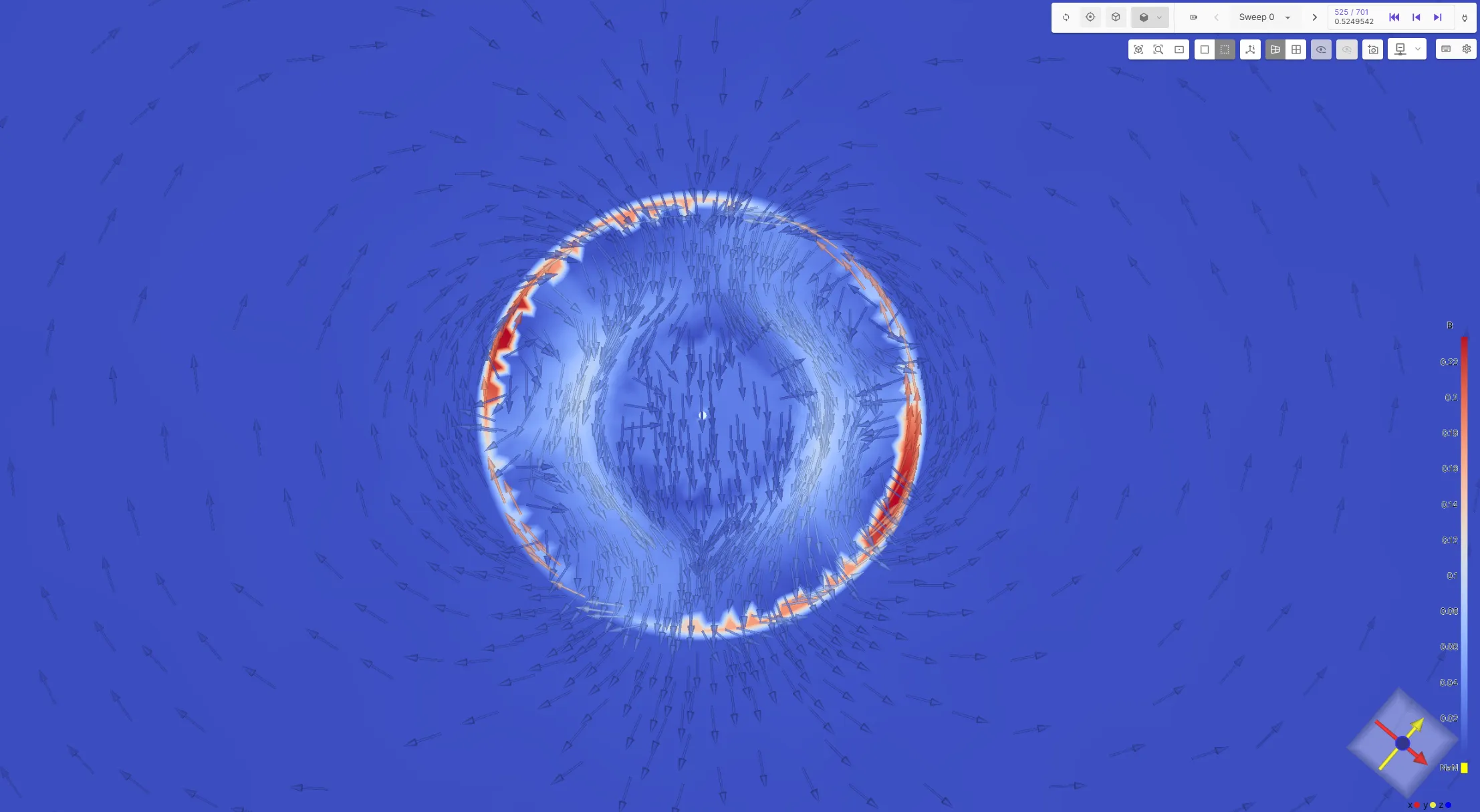
Visualization Examples
Section titled “Visualization Examples”Magnetic Flux Density B:
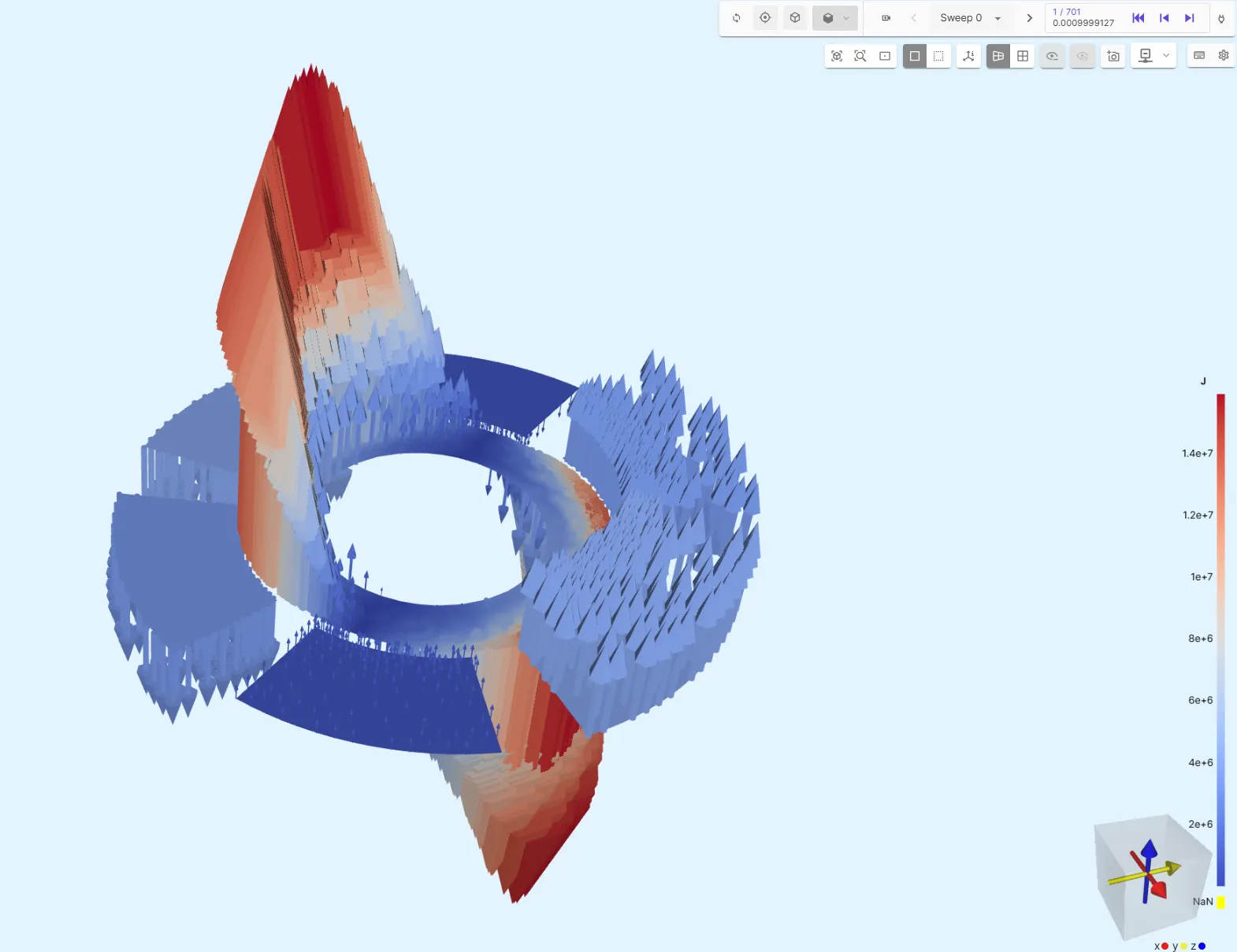
Current Density J in the windings and rotor aluminium: