SC 001 - AC losses in HTS tape demo

In this step-by-step tutorial, AC power loss in a high-temperature superconducting (HTS) tape is simulated.

HTS materials are defined as having a relatively high critical temperature of above 77 K. ¹

Model definition

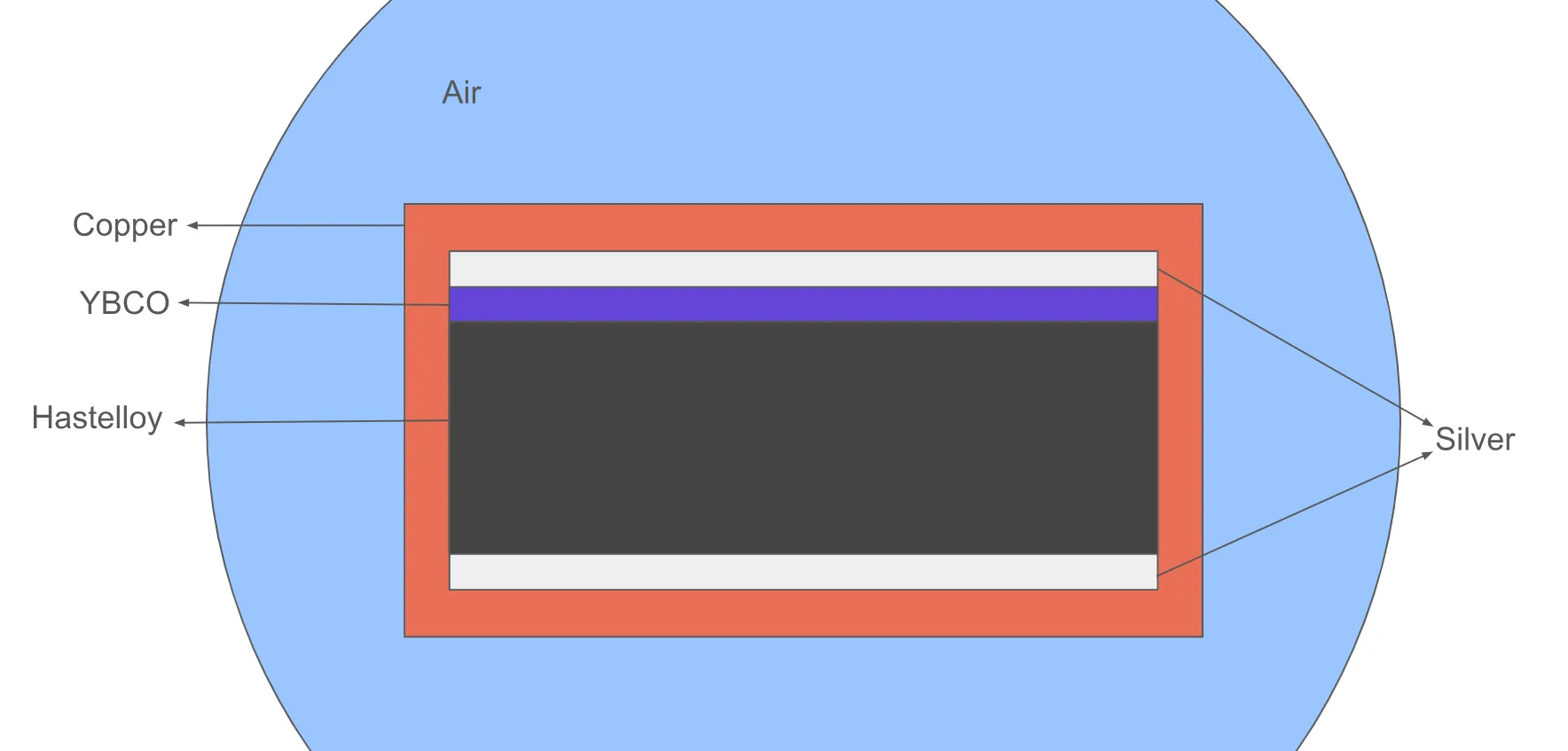
The tape model is multi-layered, with the superconducting YBCO (Yttrium barium copper oxide) layer taking up only a small part of the tape cross-section. Hastelloy is used as substrate, which forms the thick middle layer of the tape. Copper is used on the outer layer as a stabilizer.

A reference image of the tape cross-section (not to scale) as well as an image of the actual model in Allsolve model view are depicted below.

Model geometry

Element	Dimensions
air cylinder	radius = 8 cm
tape	width = 4 mm, height = 95 μm, length = 1 cm
copper layer	thickness = 20 μm
silver layer	thickness = 2 μm
YBCO layer	thickness = 1 μm
hastelloy layer	thickness = 50 μm
domain	length = 1 cm
YBCO cross-section	$A_{\rm YBCO}$ = $3.96 \cdot 10^{-9}$ m²

Material Data

Magnetic permeability ($\mu$)

• all domains: $\mu_0$

Electric resistivity ($\rho$)

• Hastelloy: $10^{-6}~\Omega$m
• Silver: $10^{-8}~\Omega$m
• Copper: $10^{-8}~\Omega$m
• YBCO:
  • $\rho=\frac{E_c}{J_c}\left(\frac{||J||}{J_c} \right)^{n-1}$
    • $E_c = 100$ μV/m
    • $n=30.5$
    • $J_c=2.85\times 10^{10}$ [A/m$^2$]
    • $I_c=J_c\cdot A_{\rm YBCO}$
  • $E\approx E^0+\frac{\partial E}{\partial J}(J-J^0)$

Inputs - case 1

• Frequency $f=50$ Hz

• Operation current $I_{\rm op}(t) = 0.8 ~ I_c \cdot \sin (2 \pi f t)$

• External magnetic flux density $B_{\rm ext}(t)=0$ [T]

Inputs - case 2

• Frequency $f=50$ Hz

• Operation current $I_{\rm op}(t)=0$ A

• External magnetic flux density $B_{\rm ext}(t) = 20 \cdot \sin (2 \pi f t)$ [mT]

Output results

• Joule losses in the YBCO region, and in the normalconducting region

$$\begin{equation} P_i(t)=\int_{\Omega_{i}}\boldsymbol{E}(t)\cdot \boldsymbol{J}(t)~\rm{d}\Omega \end{equation}$$

• Field visualizations

Step-by-step guide

Here you’ll find a detailed step-by-step tutorial on how to simulate AC Loss in an HTS tape in Quanscient Allsolve.

Step 1 - Create the project and import geometry

1. Create a new project and name it as HTS tape demo.

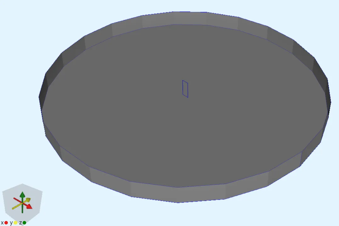
2. Import the model as a mesh file. You can download the file here: htstape.msh

The air cylinder takes up most of the model view, with the small rectangular tape volume visible in the middle.

Step 2 - Define shared regions

1. Go to the Properties section.

2. Define shared regions:

   Region name	Region type	Target
   air	Volume	volume 5
   copper	Volume	volume 6
   silver	Volume	volumes 1, 4
   hastelloy	Volume	volume 2
   ybco	Volume	volume 3
   tape	Volume	volumes 1 - 4, 6
   normalconducting	Volume	volumes 1, 2, 4, 6

   Tip: Text-based target picking

   It’s easiest to define these shared regions by picking tags as targets, as selecting thin layers in the model view can be laborious.

   Text-based target picking is especially useful, as it allows copy-pasting tag lists directly:

   

3. Define these Surface shared regions at the end of the tape:

   Region name	Region type	Target
   s_copper	Surface	surface 32
   s_silver	Surface	surfaces 13, 25
   s_hastelloy	Surface	surface 17
   s_ybco	Surface	surface 21
   s_tape	Surface	surface 13, 17, 21, 25, 32

Step 3 - Define the materials

1. Assign the predefined Air, Silver, Copper and YBCO materials to their corresponding shared regions.

2. In material properties, change Electric conducticity for Silver and Copper to 1e8.

3. Change the YBCO material color to purple in order to distinguish it from Hastelloy.

4. Create the new material Hastelloy and add its properties:

   Material name	Color	Target
   Hastelloy	Dark grey	hastelloy region (volume 2)

   Material Property	Value
   Electric conductivity	1e6
   Magnetic permeability	mu0

Step 4 - Define shared expressions

1. Edit predefined shared expressions:

   Name	Updated expression
   YBCO_Jc	2.85e10
   YBCO_n	30.5

2. Define new shared expressions:

   Name	Expression
   freq	50
   Bext	0
   Aybco	3.96e-9
   Iop	0.8 * YBCO_Jc * Aybco * sin(2 * pi * freq * t)

Step 5 - Define physics and boundary conditions

Add to the Physics section.

Add the Magnetism φ and Magnetism H physics before moving on to set up their interactions.

Physics 1 - Magnetism φ

1. Set the Magnetism φ target:

   Physics	Target
   Magnetism φ	air region (volume 5)

2. Add a constraint interaction to Magnetism φ:

   Interaction name	Interaction type	Target	Value
   Constraint	Constraint	point at the outer edge of the air cylinder (point 26)	0

3. Add an External field interaction to Magnetism φ:

   Interaction name	Interaction type	Target	Value
   External field	External field	outer surface of the air cylinder (surface 26)	[0; Bext; 0]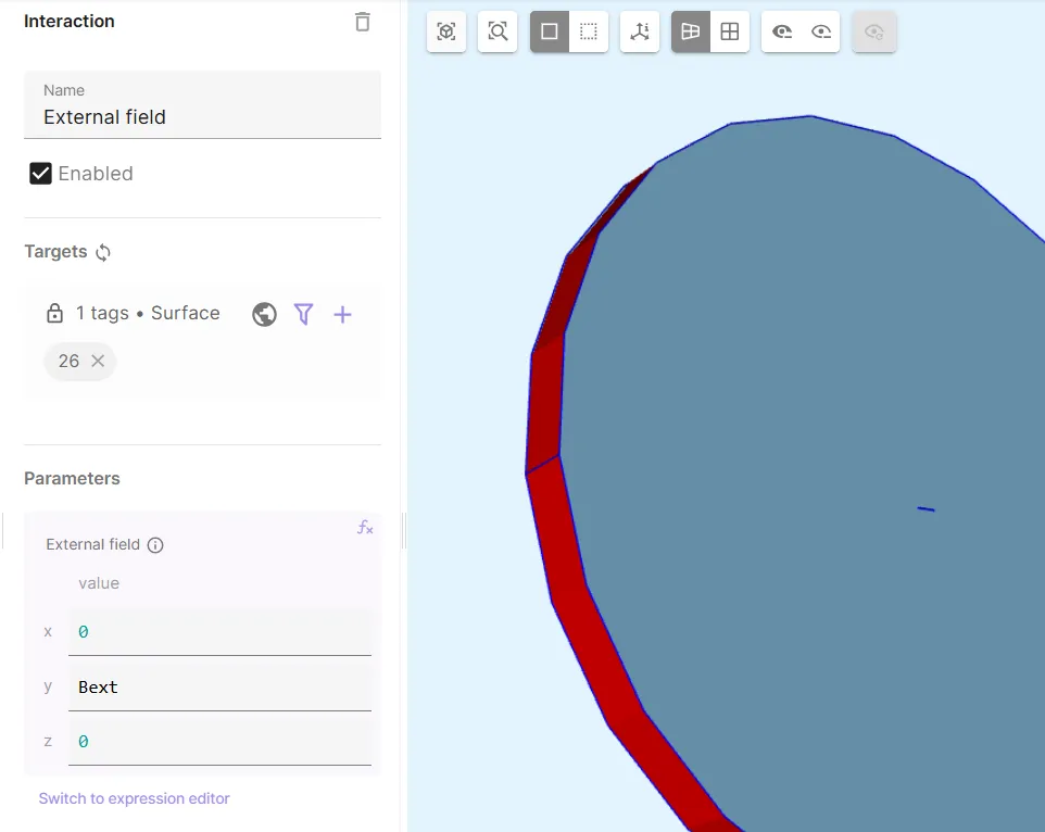

   

4. Add a Lump I/V cut interaction to Magnetism φ:

   Interaction name	Interaction type	Target	Actuation mode	Current
   Lump I/V cut	Lump I/V cut	a loop around the tape cross-section (curves 46, 48, 50, 51)	Current	Iop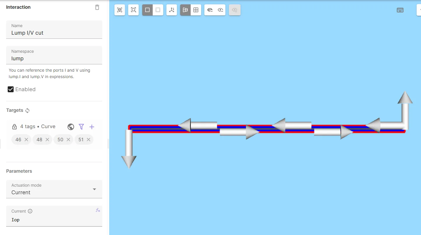

   

Physics 2 - Magnetism H

1. Set the Magnetism H target:

   Physics	Target
   Magnetism H	tape region (volumes 1 - 4, 6)

2. Add H-φ coupling to Magnetism H.

Step 6 - Select simulation options

1. Go to the Simulations section.

2. Add a new simulation.

3. Set Analysis Type to Transient.

4. Set Timestep algorithm to Implicit Euler.

5. Set Start time to 0 [s].

6. Set End time to 0.02 [s].

7. Set Timestep size to 0.001 [s].

8. Set Solver mode to Direct solver.

9. Select the imported mesh as the mesh for your simulation.

Step 7 - Add simulation outputs

1. Add custom value outputs for joule loss integrals:

   Name	Output expression
   Pybco	integrate(reg.ybco, transpose(E)*j, 2)
   Pnc	integrate(reg.normalconducting, transpose(E)*j, 2)

2. Add custom value outputs for net currents:

   Name	Output expression
   Itot	lump.I
   Iybco	integrate(reg.s_ybco, on(reg.ybco, compz(j)), 2)

3. Add the j field output with ybco region as target (volume 3).

4. Toggle Skin only on the j field output.

Step 8 - Modify the simulation script & run

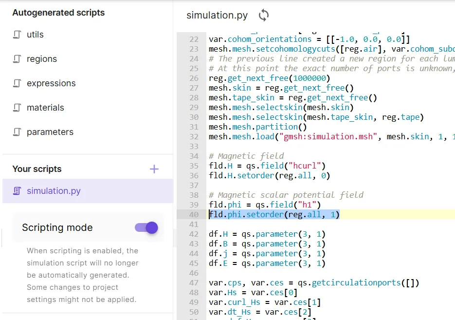
1. Open the simulation Script.

2. Enable Scripting mode.

3. Change the φ interpolation order to 1.

4. Replace the first line of the autogenerated magnetism H formulation with the following Newton-Raphson linearization:

   rho = 1 / par.sigma(df.j)
   dedj = rho * qs.eye(3) + (expr.YBCO_n - 1.0) * rho / qs.max(df.j * df.j, 1e-40) * df.j * qs.transpose(df.j)
   dofe = rho * df.j + dedj * (qs.curl(qs.dof(fld.H)) + var.curl_dof_Hs - qs.curl(fld.H) - var.curl_Hs)
   form += qs.integral(reg.ybco, dofe * (qs.curl(qs.tf(fld.H)) - var.curl_tf_Hs))
   form += qs.integral(reg.normalconducting, qs.inverse(par.sigma(df.j)) * (qs.curl(qs.dof(fld.H)) + var.curl_dof_Hs) * (qs.curl(qs.tf(fld.H)) - var.curl_tf_Hs))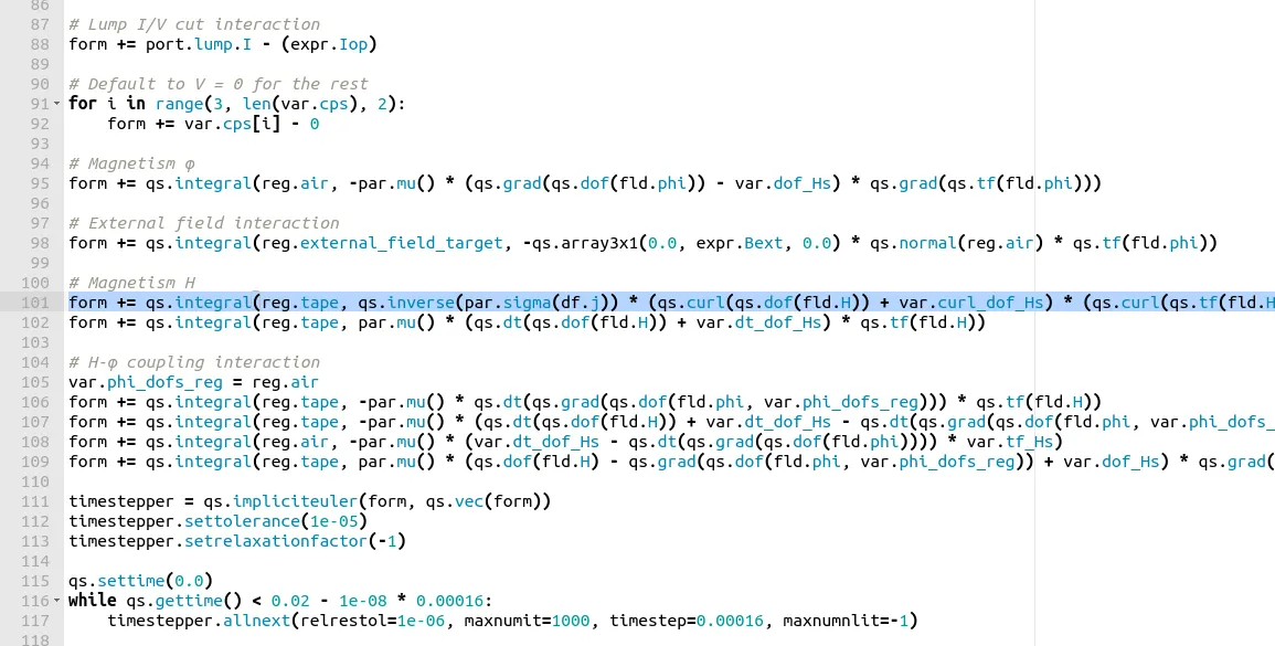

   

   The Newton-Raphson linearization helps in speeding up the convergence of nonlinear systems, leading to faster runtimes. In some cases, the nonlinear system does not converge at all with fixed point iteration unless linearized.

5. Change timestepper tolerance to 1e-4 and j field output region to reg.s_ybco.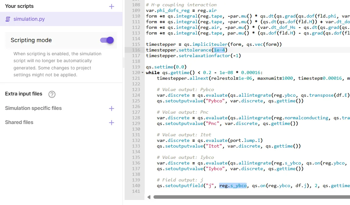

   

6. Save the script.

7. Run the simulation.

Step 9 - Visualize results

1. Add a visualization for the j field.

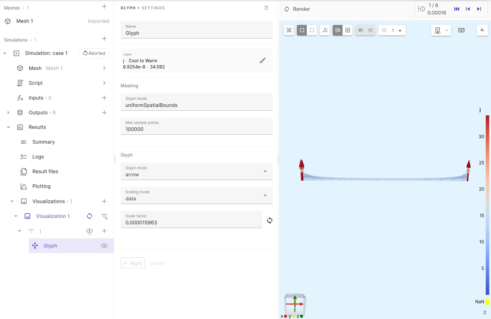
2. Add Glyph to the j field visualization with options as below.

References

Footnotes

1. https://en.wikipedia.org/wiki/High-temperature_superconductivity ↩