Inputs

In Quanscient Allsolve, simulations can be run without any additional inputs. However, they provide additional versatility in setting up a simulation.

There are 3 types of simulation inputs in Quanscient Allsolve:

• Overrides
  • Override a shared expression with a single value
• Sweeps
  • Override a shared expression with a vector of values, running a simulation sweep
• Field initializations
  • Initialize a simulation with a field state from a previous simulation

To create an input for a simulation, click + next to Inputs:

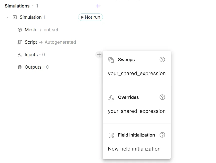
Next, we’ll take a closer look at each of the 3 input types.

Overrides

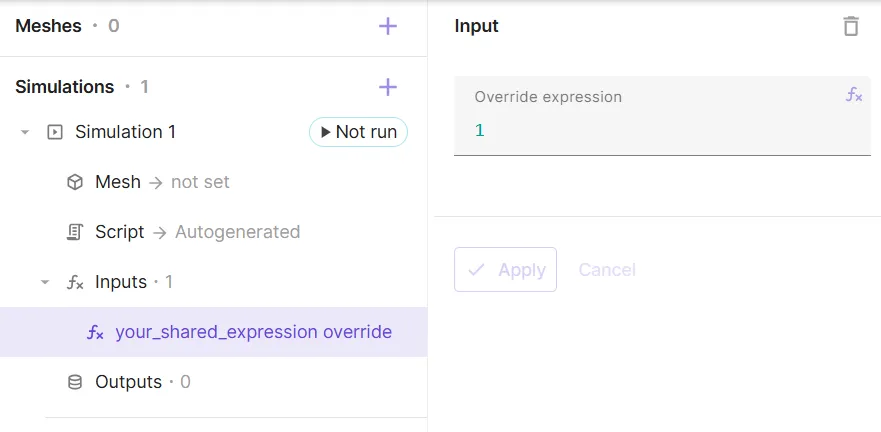
In some cases, you might want to modify the value of a shared expression only for the runtime of a specific simulation. Allsolve allows you to override a shared expression, changing the value for the runtime of a simulation.

To override a shared expression, add an override to Inputs and define the override expression:

Caution: Geometry dimensions and overrides

Shared expressions used as geometry dimensions cannot yet be used in overrides.

Caution: Overrides and sweeps

Overrides and sweeps cannot be used in the same simulation on the same shared expression.

Sweeps

Sweeps are an extension of overrides, allowing a vector of override values to be used as the override expression. A sweep is a series of subsimulations - one subsimulation for each value in the override vector. A sweep with a single value in the override vector is identical to an override:

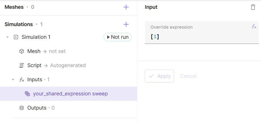
With sweeps, you can easily run multiple variations of your model in one go, varying one or more parameters. Parameters to be swept over must be defined as shared expressions.

Caution: Geometry dimensions and sweeps

Shared expressions used as geometry dimensions cannot yet be used in sweeps. Geometric sweeps are in the works!

Caution: Overrides and sweeps

Overrides and sweeps cannot be used in the same simulation on the same shared expression.

1-variable sweeps

Defining override vectors for univariate sweeps is simple.

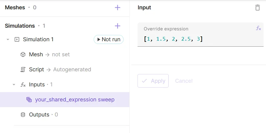
1. Small vectors can be entered in square brackets, []:

   

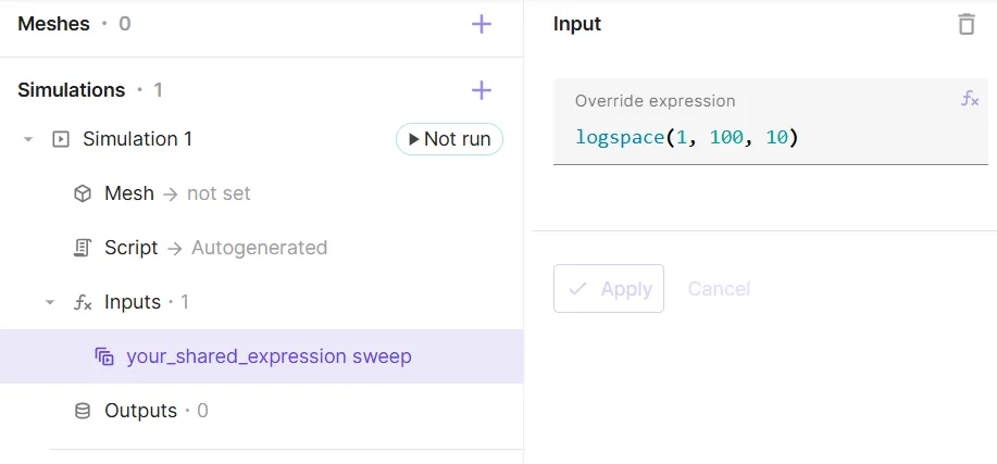
2. Larger vectors can be entered using the linspace or logspace functions: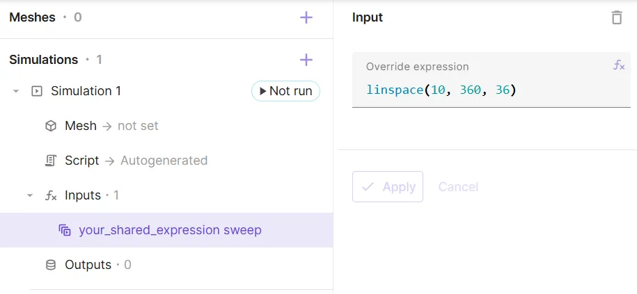

   

   

2-variable sweeps

Multivariate sweeps run by aligning indices between override vectors, so that subsimulation i takes the value in index i of each override vector. For this reason, when using multiple sweep parameters in the same simulation, the override vector lengths must match.

For example, consider a solid mechanics simulation intended to run for the following list of pairs of Young’s modulus E and Poisson’s ratio nu:

(150e9, 0.2), (150e9, 0.25), (160e9, 0.2), (160e9, 0.25).

To perform the sweep simulation, the following 2 sweeps are added to Inputs:

Shared expression	Override expression
E	[150e9, 150e9, 160e9, 160e9]
nu	[0.2, 0.25, 0.2, 0.25]

Note, that the length of the E and nu override expressions match (4 in this case).

Now consider a mechanical warpage sweep simulation with two variables, temperature T and coefficient of thermal expansion CTE. Assume the ranges of T = [25, 50, 75, 100, 125, 150] and CTE = [1e-6, 2e-6, 3e-6, 4e-6, 5e-6] and that it is required to run the sweep simulation for all possible resulting pairs of (T, CTE) as in the image below:

With 6 different values of T and 5 different values of CTE, this results in a total of 6 x 5 = 30 pairs of (T, CTE). The override expressions with 30 elements each are provided as follows:

Shared expression	Override expression
T	[25,25,25,25,25, 50,50,50,50,50, 75,75,75,75,75, 100,100,100,100,100, 125,125,125,125,125, 150,150,150,150,150]
CTE	[1,2,3,4,5, 1,2,3,4,5, 1,2,3,4,5, 1,2,3,4,5, 1,2,3,4,5, 1,2,3,4,5 ]

Providing these lists of 30 elements manually as an input can be quite tedious. If there are more than 2 variables with many different values to sweep, it becomes even more painstaking to enter all the list elements. To simplify providing these long override expression, it is recommended to use the repelem and repmat functions. For example, the same override expression as earlier for T and CTE can now be obtained with a much simpler syntax as shown below:

Shared expression	Override expression
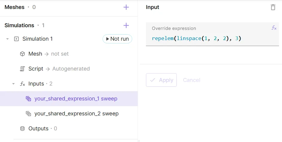
T	repelem([25, 50, 75, 100, 125, 150], 5)
CTE	repmat([1e-6, 2e-6, 3e-6, 4e-6, 5e-6], 1, 6)

As another example, let’s say you have the following 2 vectors of unique override values that you would like to create override vectors with:

Vector	Values	Length
v1	[1, 2]	l1 = 2
v2	[10, 20, 30]	l2 = 3

The override vectors can be defined with repelem and repmat as follows:

Override vector	Expression	Result
o1	repelem([1, 2], 3)	[1, 1, 1, 2, 2, 2]
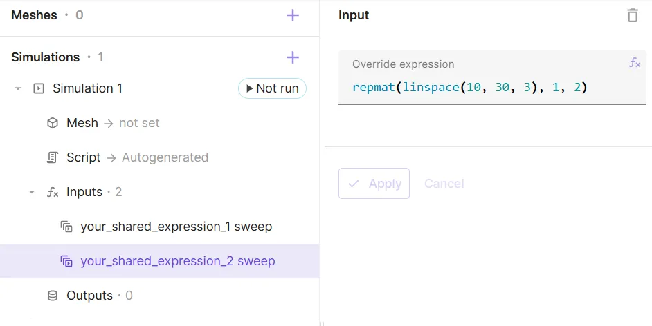
o2	repmat([10, 20, 30], 1, 2)	[10, 20, 30, 10, 20, 30]

• The last arguments of repelem/repmat are v1/v2 vector lengths.
• The second argument of repmat is always 1.
• Vectors can be entered into repelem/repmat arguments with the linspace or logspace functions:
  • 
  • 

For a generalized formula, see the table below:

Override vector	Formula
o1	repelem(v1, l2)
o2	repmat(v2, 1, l1)

3-variable sweeps

Let’s add a 3rd vector to the mix, v3:

Vector	Expression	Length
v1	[1, 2]	l1 = 2
v2	[10, 20, 30]	l2 = 3
v3	[100, 200, 300, 400]	l3 = 4

To define the override vectors, it is recommended to use a combination of the repelem and repmat functions:

Override vector	Expression
o1	repelem([1, 2], 3 * 4)
o2	repelem(repmat([10, 20, 30], 1, 2), 4)
o3	repmat([100, 200, 300, 400], 1, 2 * 3)

• The last argument of each repelem/repmat function call is based on vector lengths.
• The second argument of repmat is always 1.
• Vectors can be entered into repelem/repmat arguments with the linspace or logspace functions.

For a generalized formula, see the table below:

Override vector	Formula
o1	repelem(v1, l2 * l3)
o2	repelem(repmat(v2, 1, l1), l3)
o3	repmat(v3, 1, l1 * l2)

4-variable sweeps

Let’s add a 4th vector to the mix, v4:

Vector	Expression	Length
v1	[1, 2]	l1 = 2
v2	[10, 20, 30]	l2 = 3
v3	[100, 200, 300, 400]	l3 = 4
v4	[1000, 2000, 3000, 4000, 5000]	l4 = 5

To define the override vectors, it is recommended to use a combination of the repelem and repmat functions:

Override vector	Expression
o1	repelem([1, 2], 3 * 4 * 5)
o2	repelem(repelem(repmat([10, 20, 30], 2), 4), 5)
o3	repelem(repmat(repmat([100, 200, 300, 400], 1, 2), 1, 3), 5)
o3	repmat([1000, 2000, 3000, 4000, 5000], 1, 2 * 3 * 4)

• The last argument of each repelem/repmat function call is based on vector lengths.
• The second argument of repmat is always 1.
• Vectors can be entered into repelem/repmat arguments with the linspace or logspace functions.

For a generalized formula, see the table below:

Override vector	Formula
o1	repelem(v1, l2 * l3 * l4)
o2	repelem(repelem(repmat(v2, l1), l3), l4)
o3	repelem(repmat(repmat(v3, 1, l1), 1, l2), l4)
o3	repmat(v4, 1, l1 * l2 * l3)

You might see a pattern emerging at this point. You’re not likely to need more than 4 override vectors in any simulation, but if you do, the vector definitions will follow the same logic of combining repelem/repmat.

Field initializations

Field initializations can be used to initialize a simulation with a final field state from a previous simulation. To use a field initialization, add a final field state output to an existing simulation and run it.